Incomplete markets as a complementary channel for emerging-market volatility.
Heterogeneous Agents & Cross-Section
Herreño & Pedemonte 22', Hong 23', Guntin et al. 23'
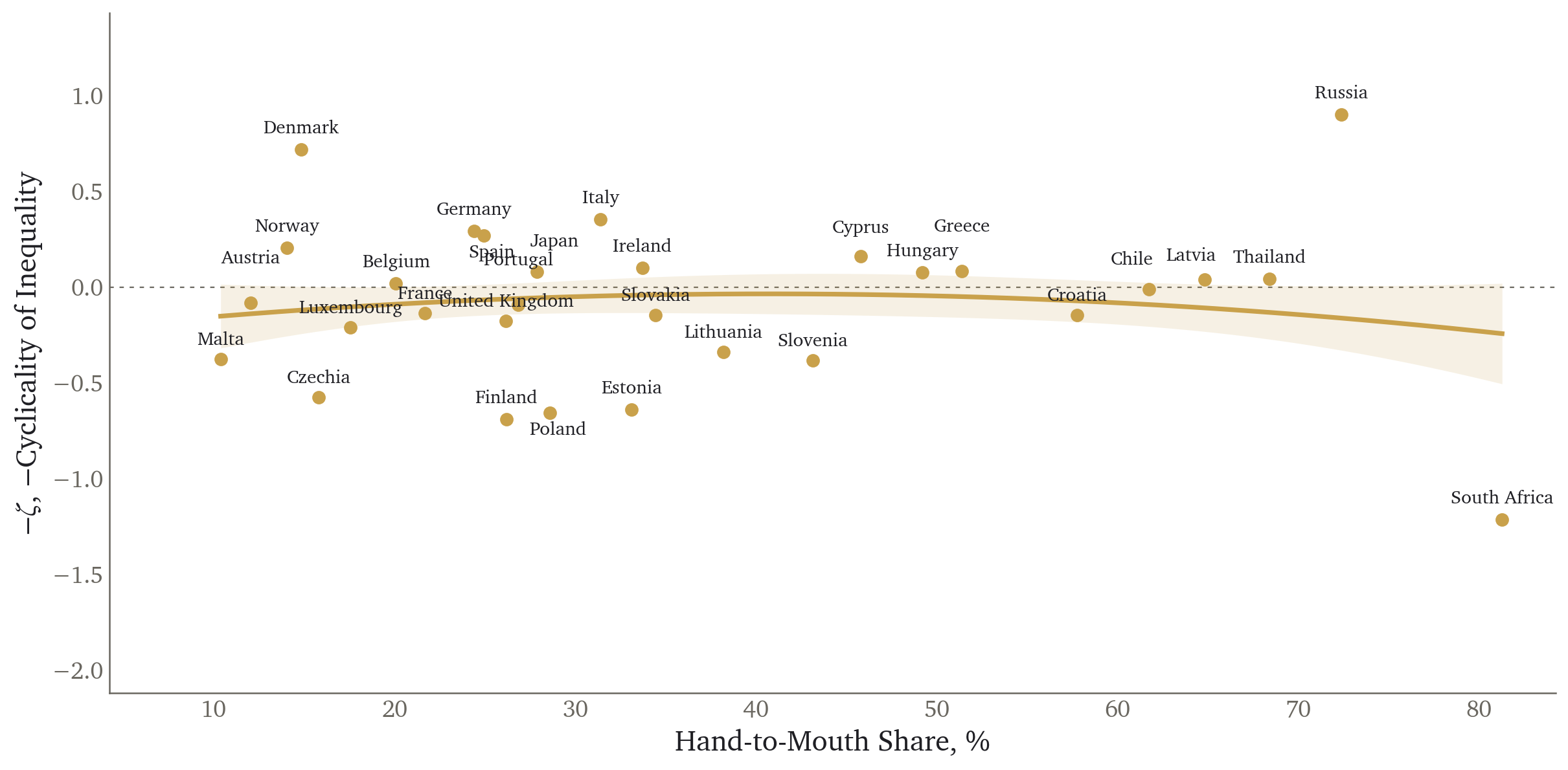
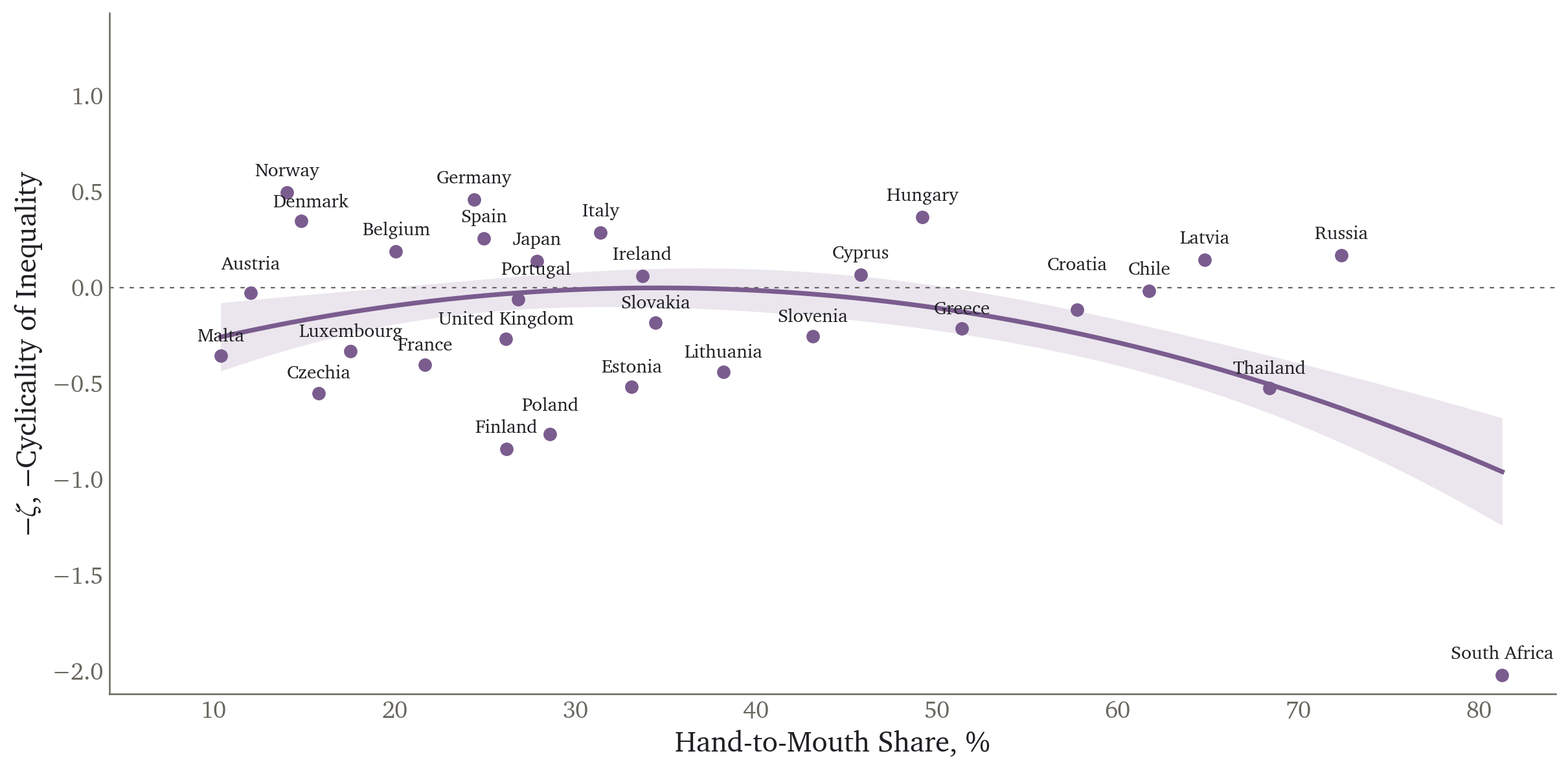
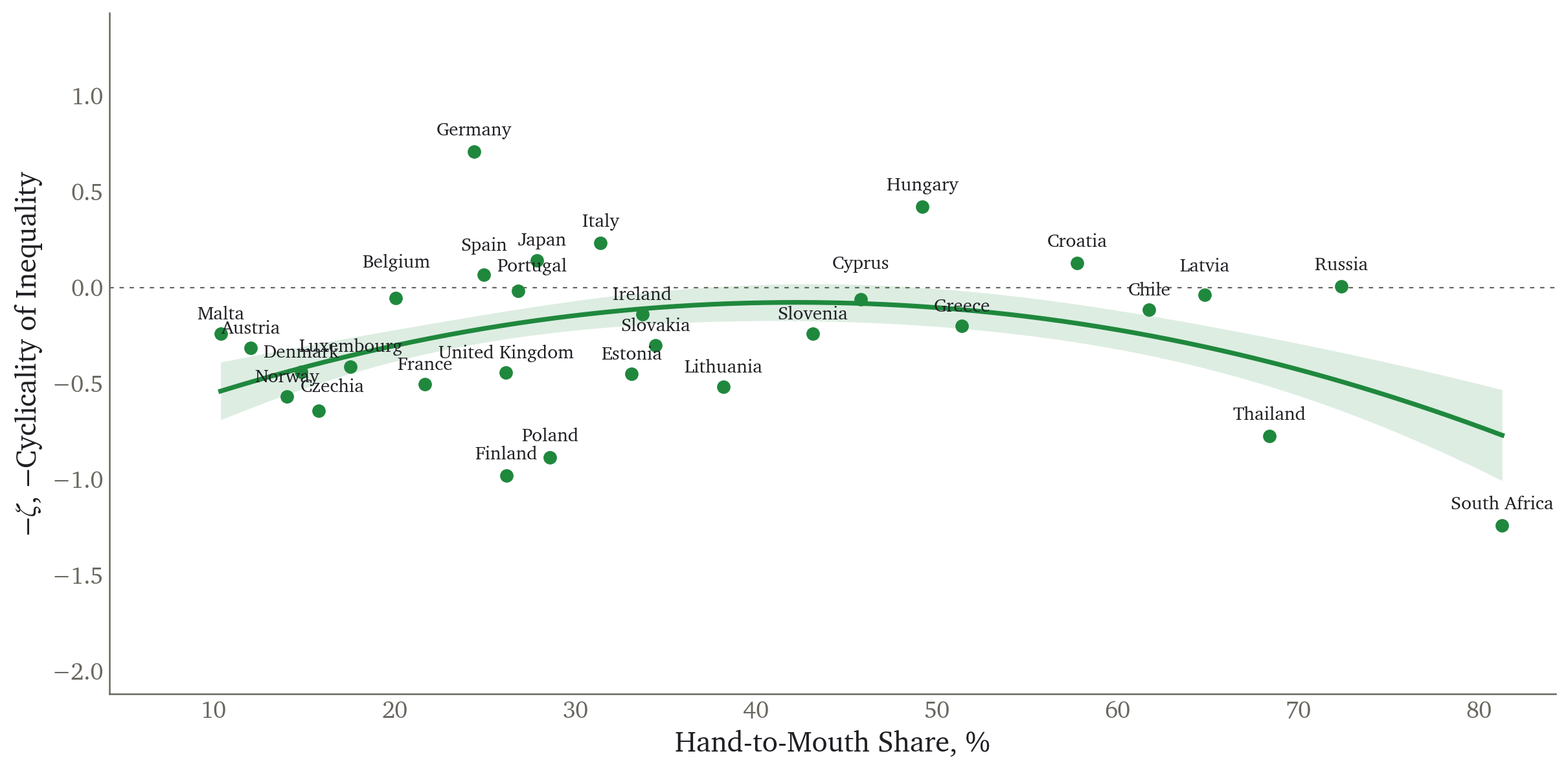
Isolate countercyclical inequality and income risk as the mechanism.
Empirics
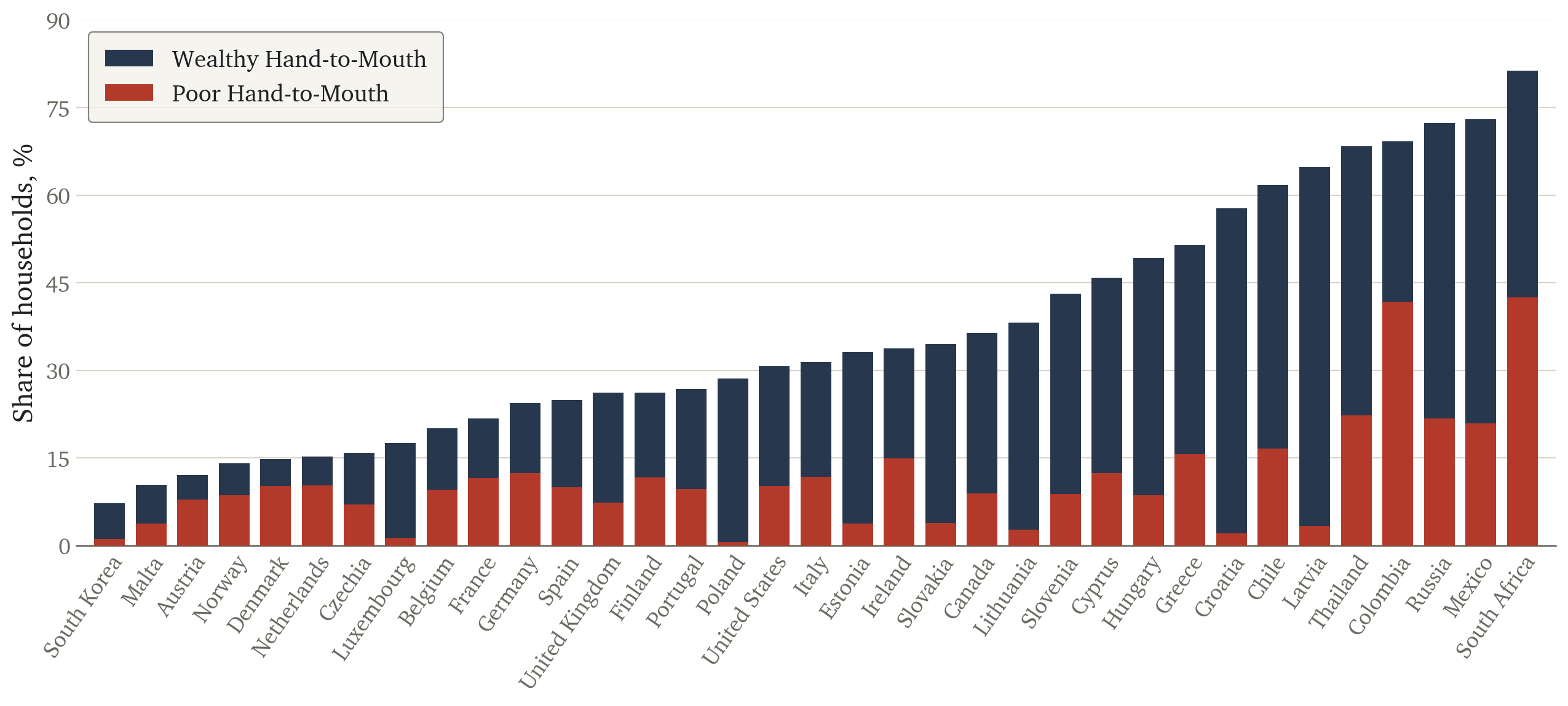
Hand-to-Mouth Shares Data
Household-level finance surveys
Assets, liabilities, income, consumption and demographics for 35 countries, yearly, circa 2017
Canada: Survey of Financial Security (SFS) ·
Chile: Encuesta Financiera de Hogares (EFH) ·
Colombia: Encuesta de Carga Financiera y Educación Financiera (IEFIC) ·
Denmark: Wealth and other Administrative Registers ·
European Union: Household Finance and Consumption Survey (HFCS) ·
Mexico: Encuesta Nacional sobre las Finanzas de los Hogares (ENFIH) ·
Norway: Household Wealth Statistics ·
Russia: Russia Longitudinal Monitoring Survey (RLMS-HSE) ·
South Africa: National Income Dynamics Study (NIDS) ·
South Korea: Survey of Household Finances and Living Conditions (SFLC) ·
Thailand: Townsend Thai Survey (TTS) ·
United Kingdom: Wealth and Assets Survey (WAS) ·
United States: Survey of Consumer Finances (SCF)
with $\mathbf{S}\mathbf{I}\mathbf{S}' = \boldsymbol{\Sigma}$ and $\boldsymbol{\epsilon}_t = [\epsilon_{ip,t},\, \epsilon_{p,t},\, \epsilon_{ur,t},\, \epsilon_{r,t}]$. The system is identified if
where $\boldsymbol{X}_{t-1}$ is a vector of the changes over the 65 trading days
before the meeting in the equity index, the exchange rate, the sovereign yields, the VIX
and a commodity index.
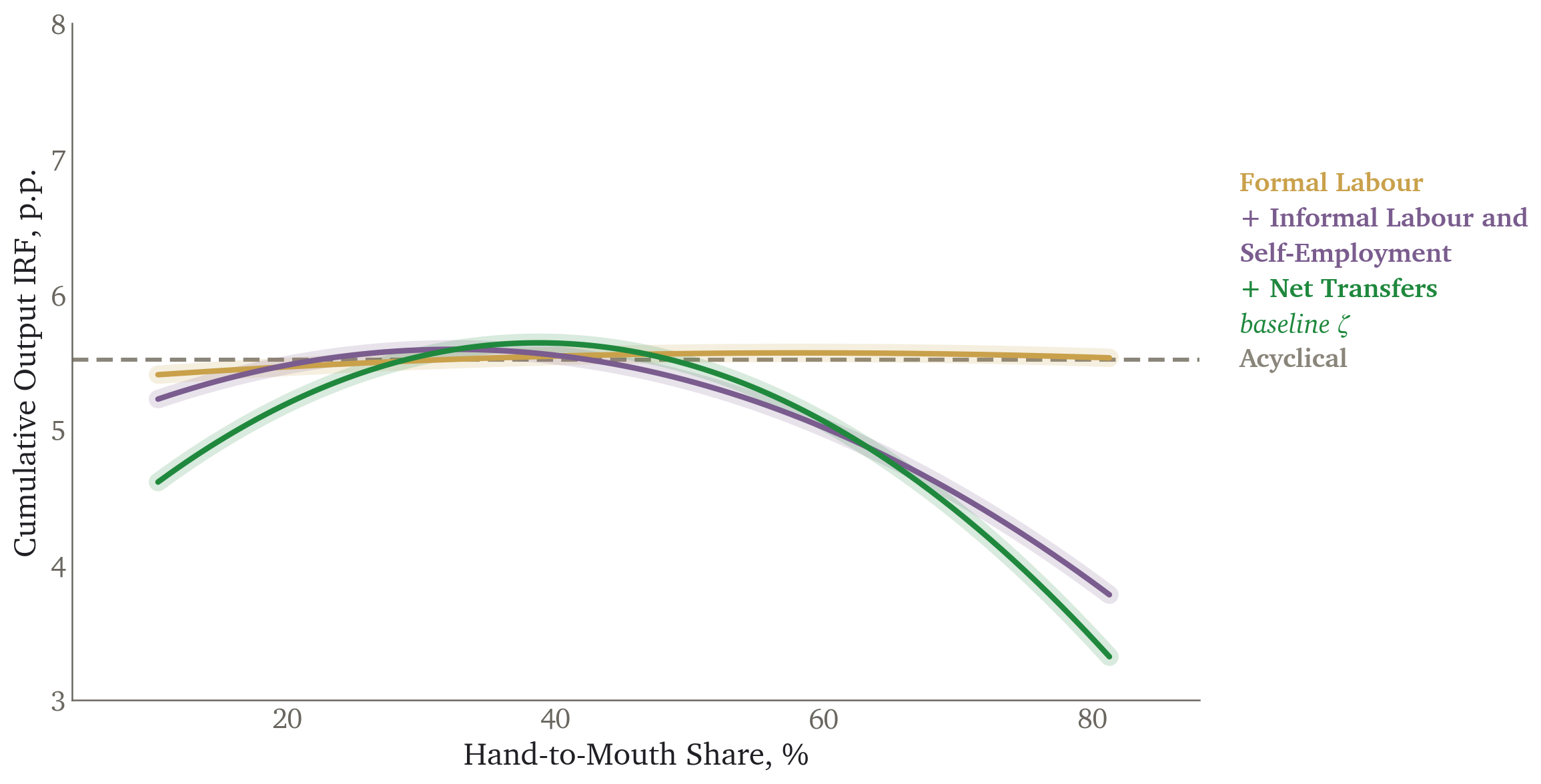
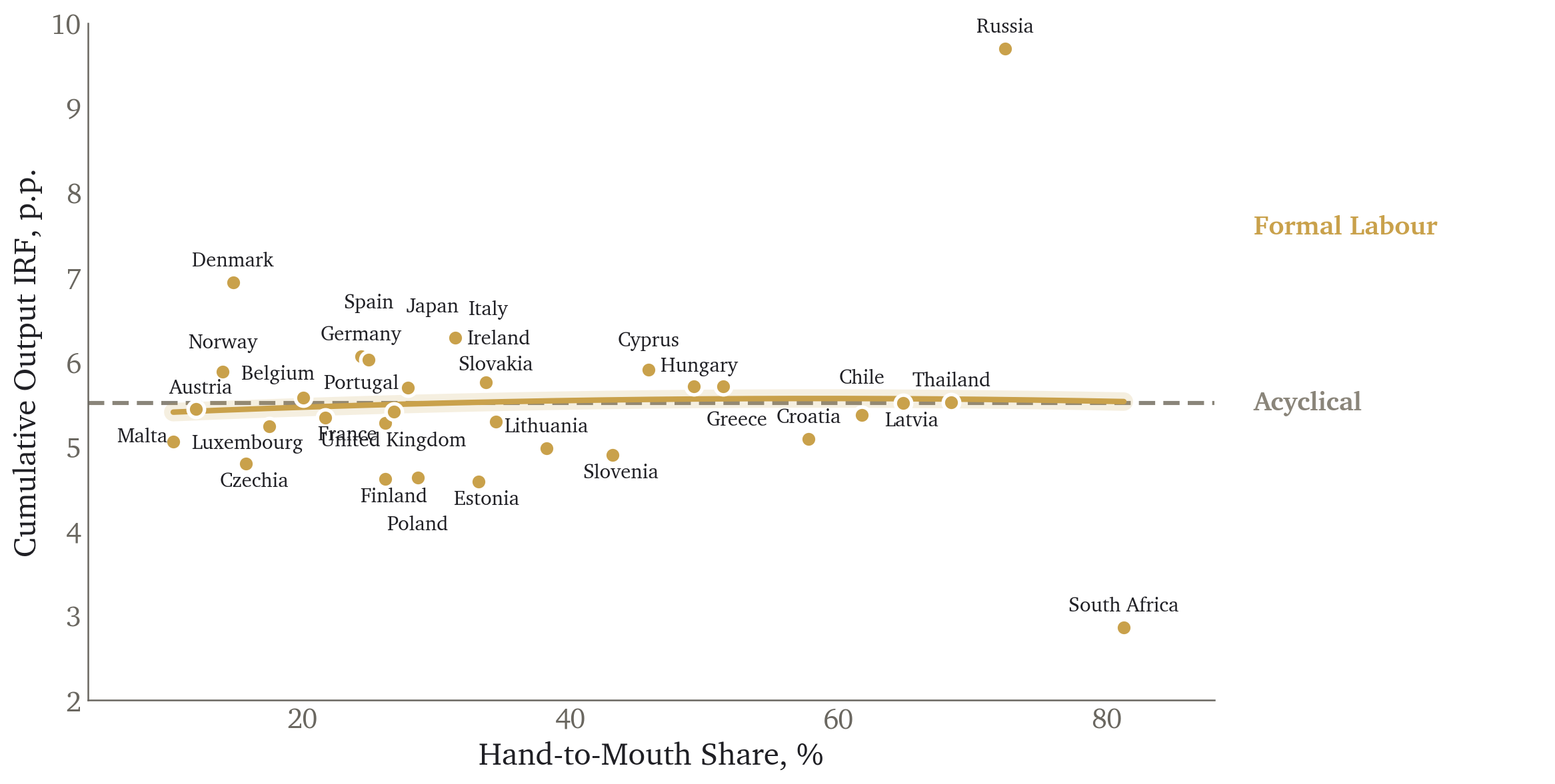
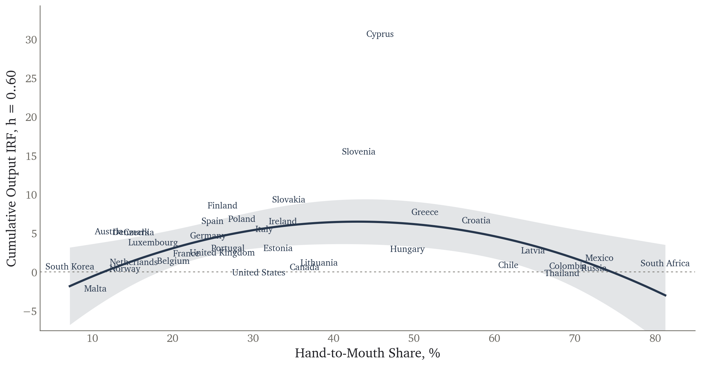
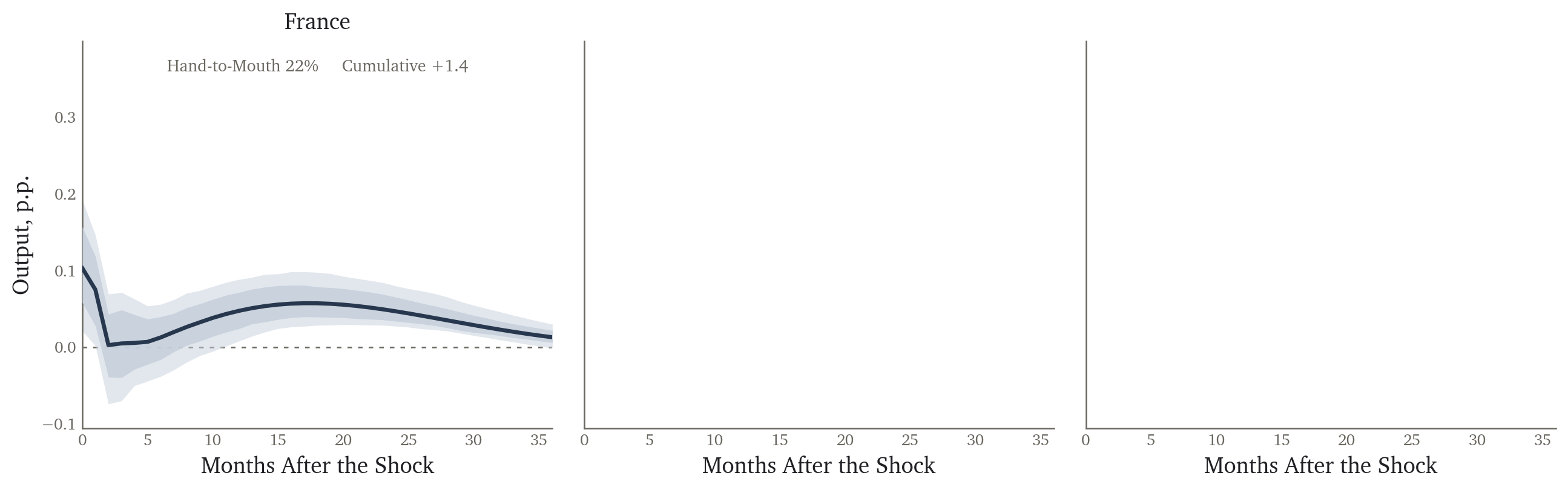
Output Responses to Monetary Shocks IRFs
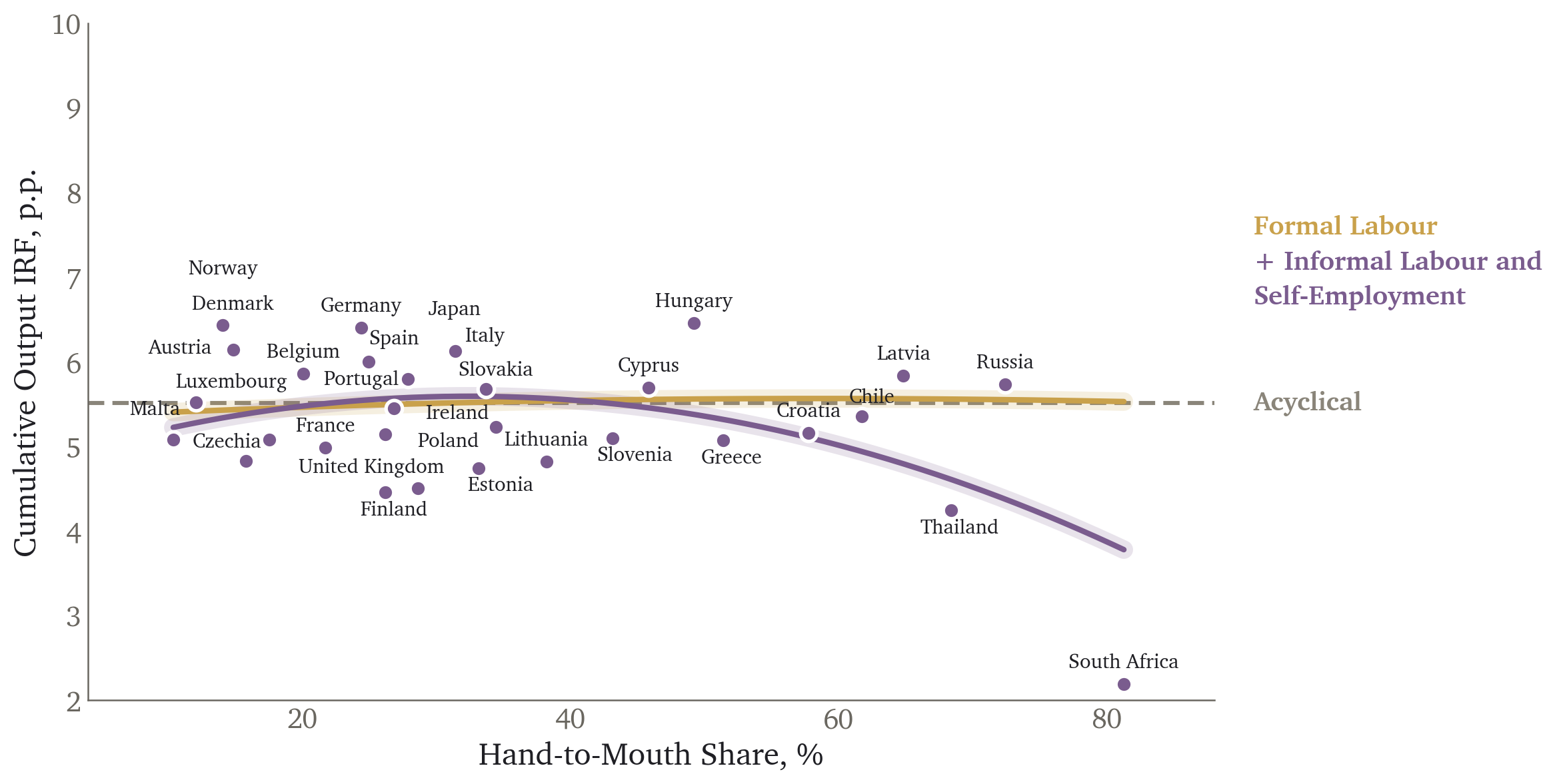
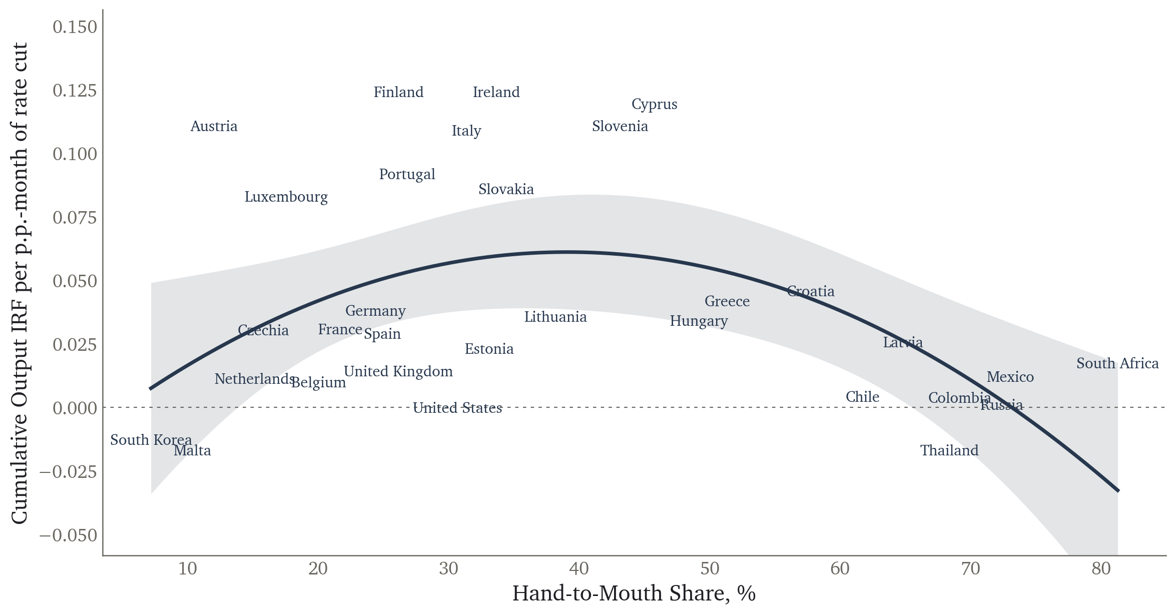
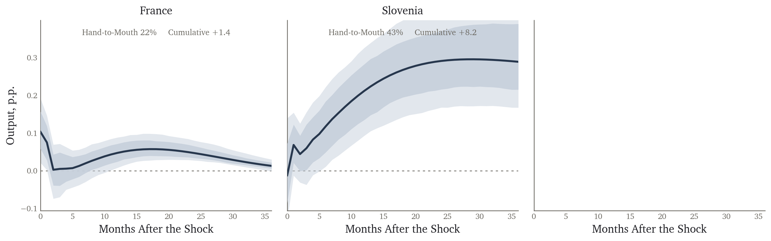
Output Responses to Monetary Shocks IRFs
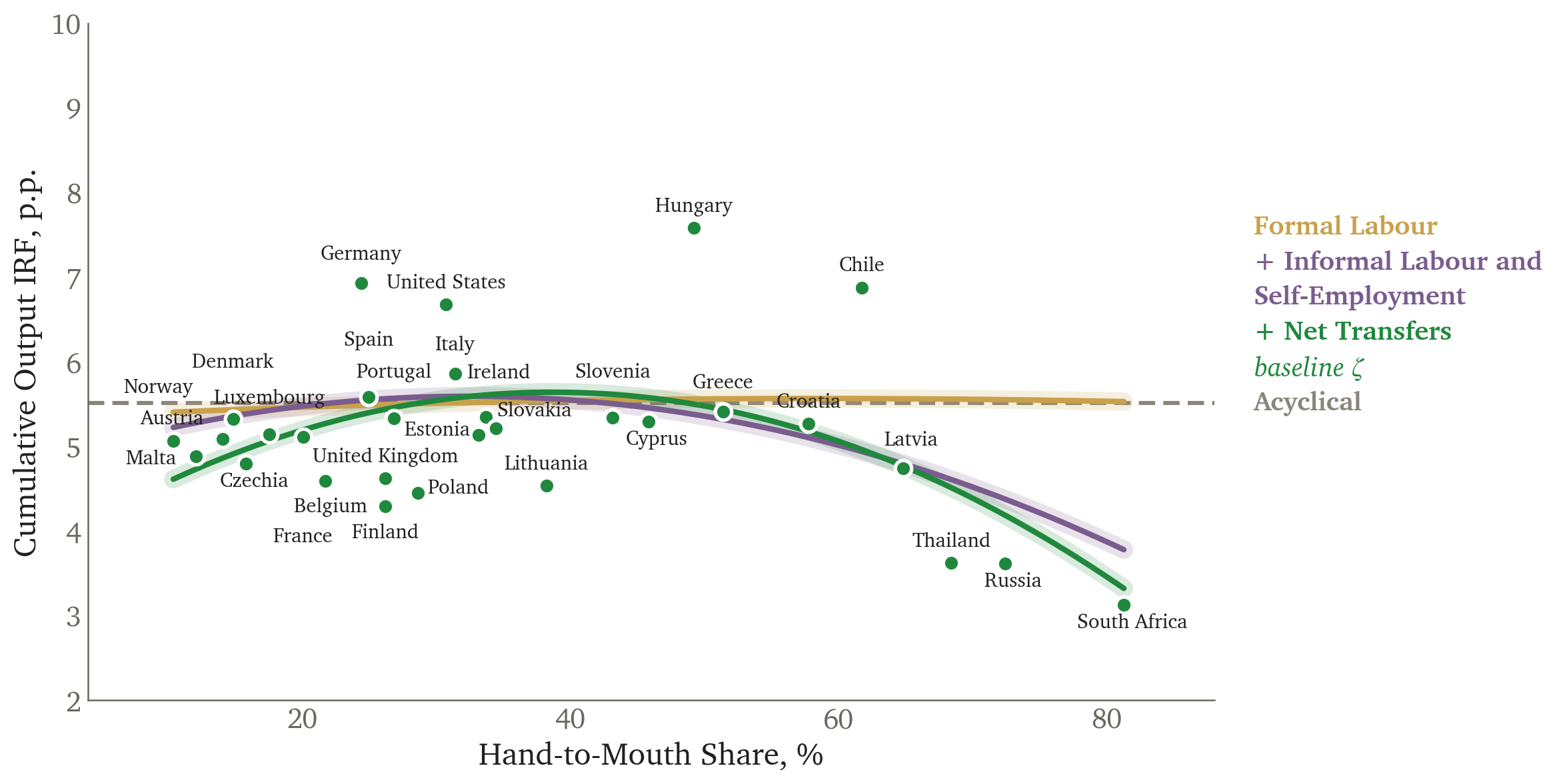
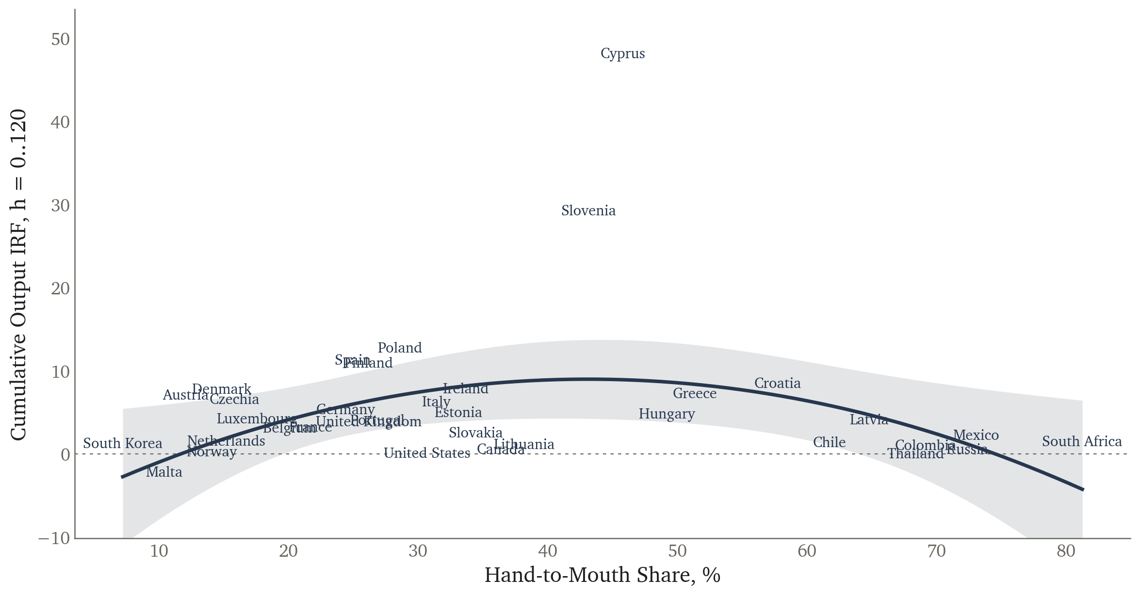
Output Responses to Monetary Shocks IRFs
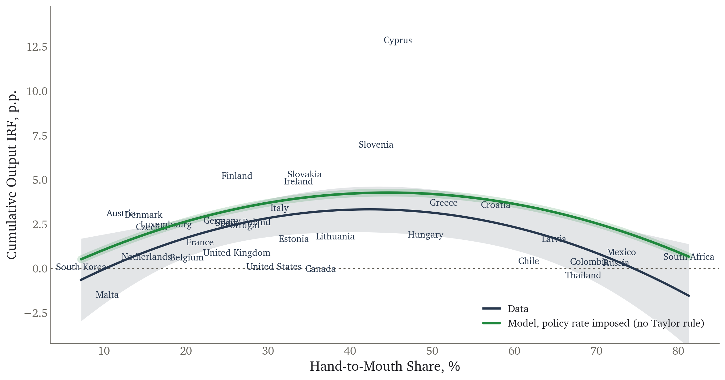
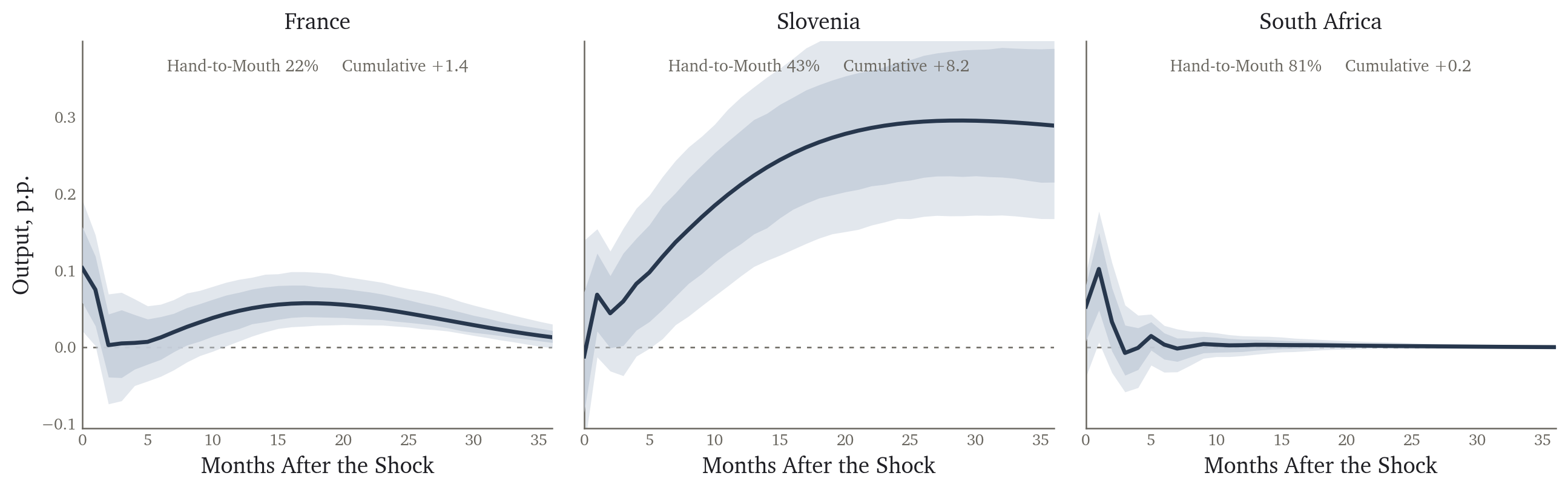
Output Responses to Monetary Shocks IRFs
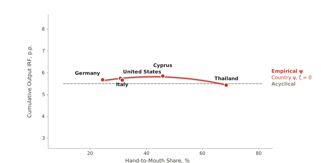
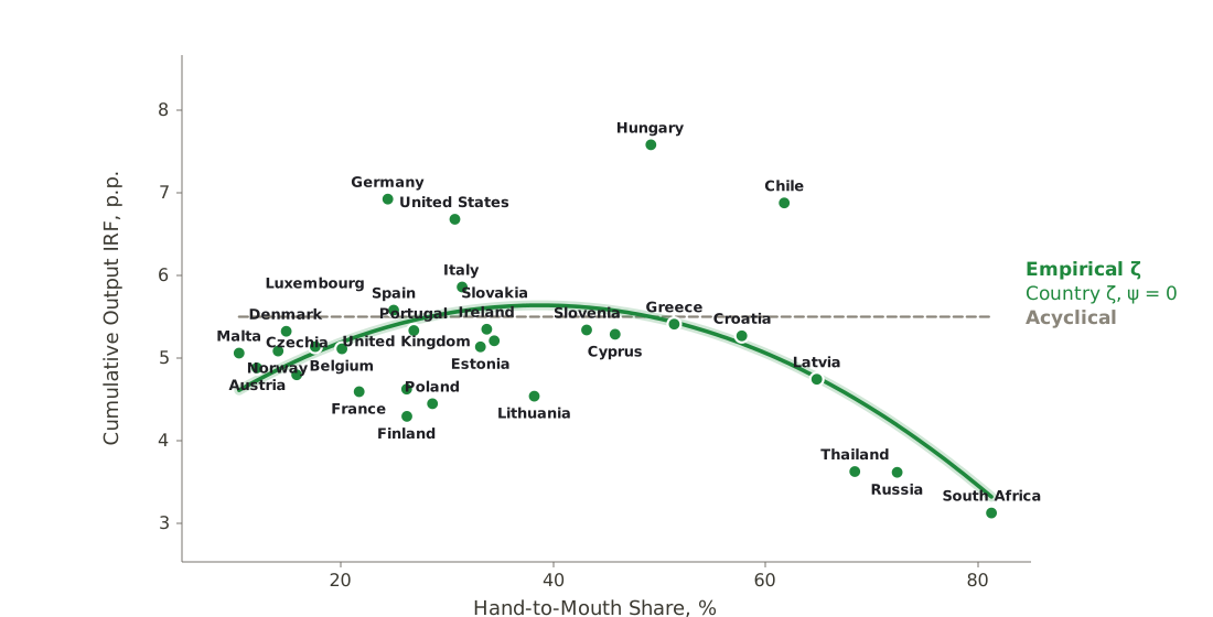
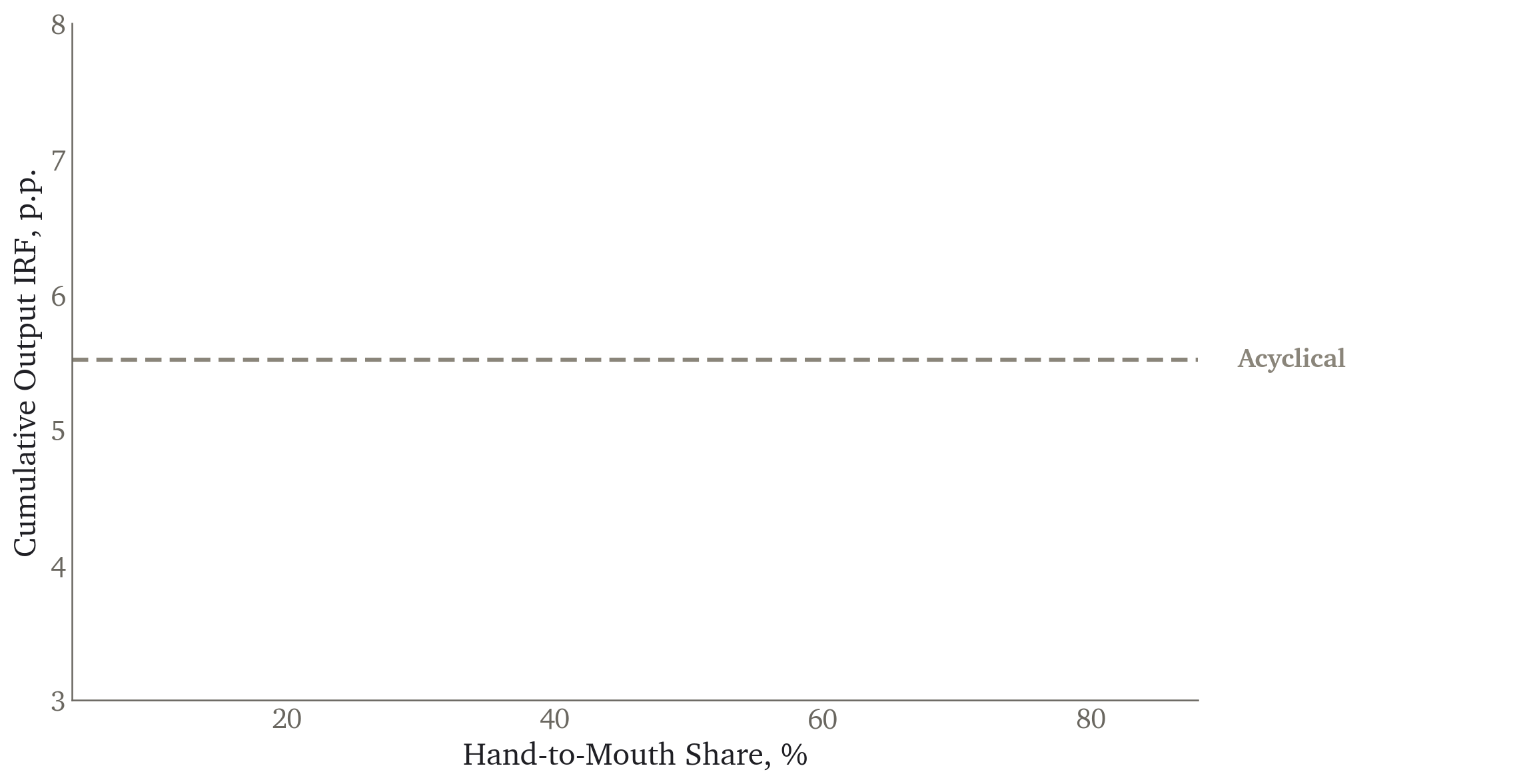
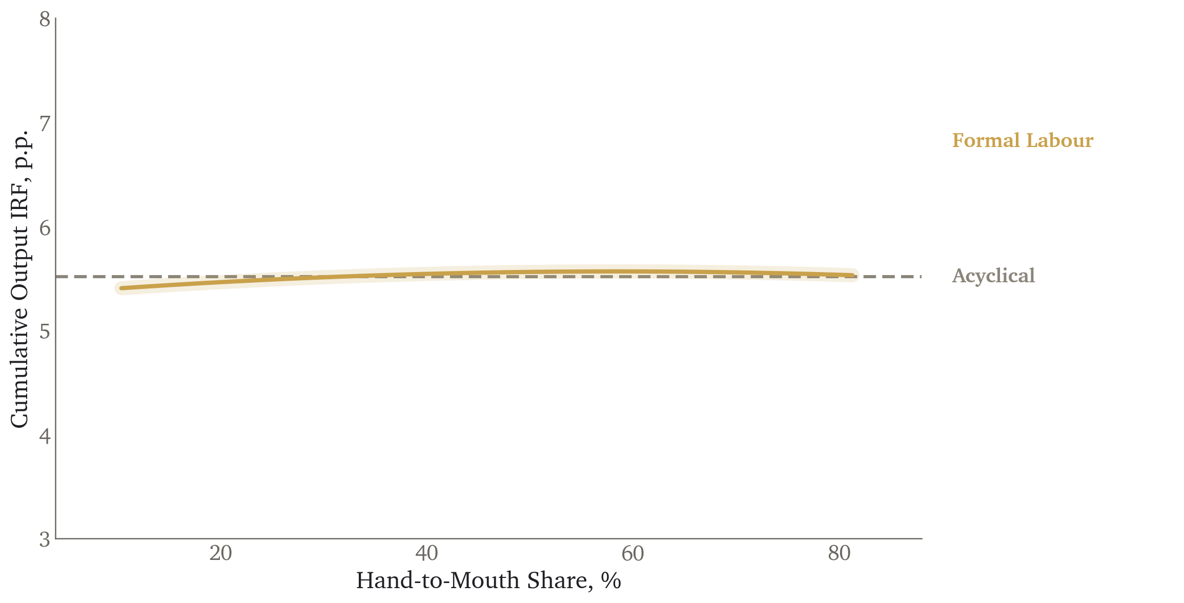
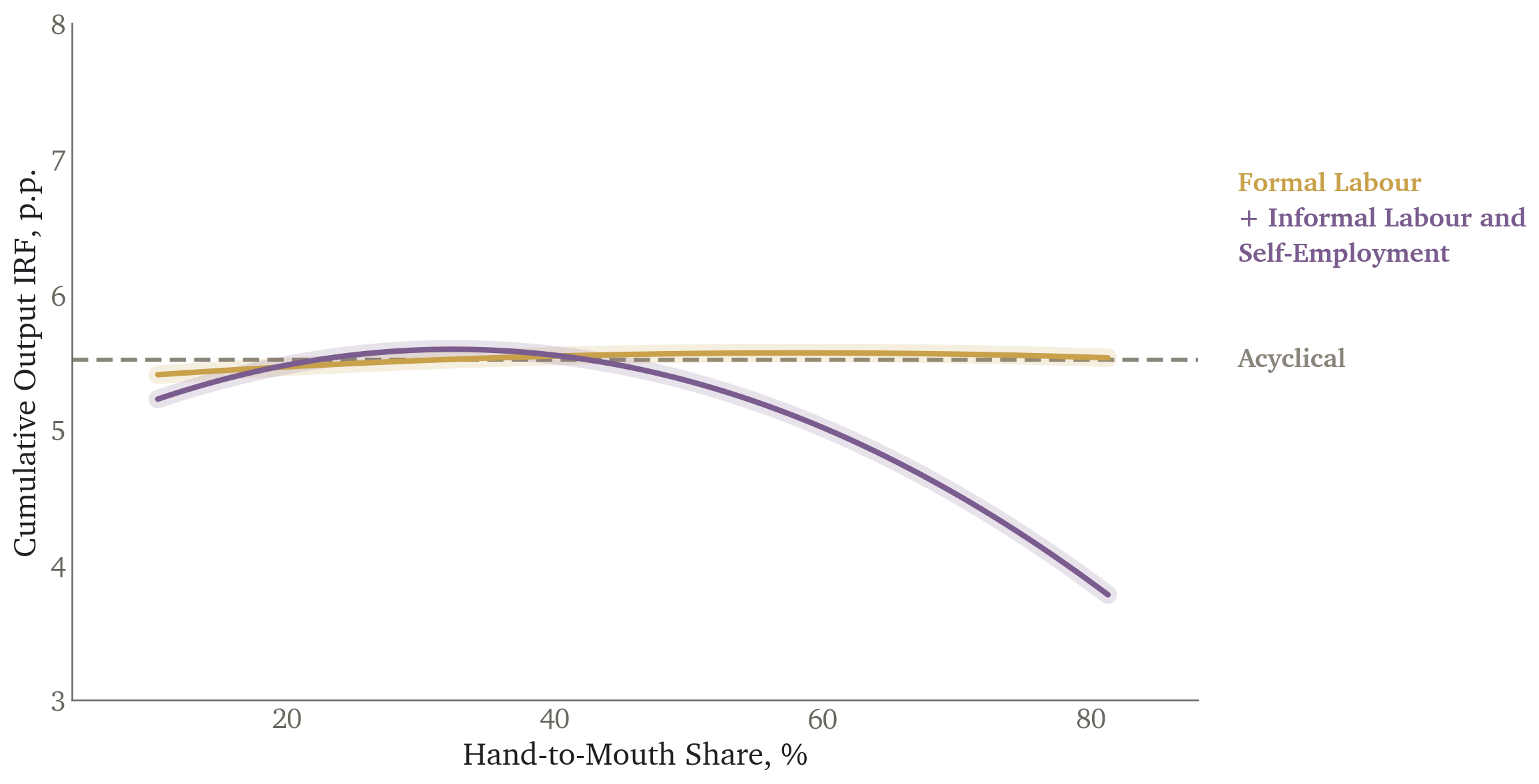
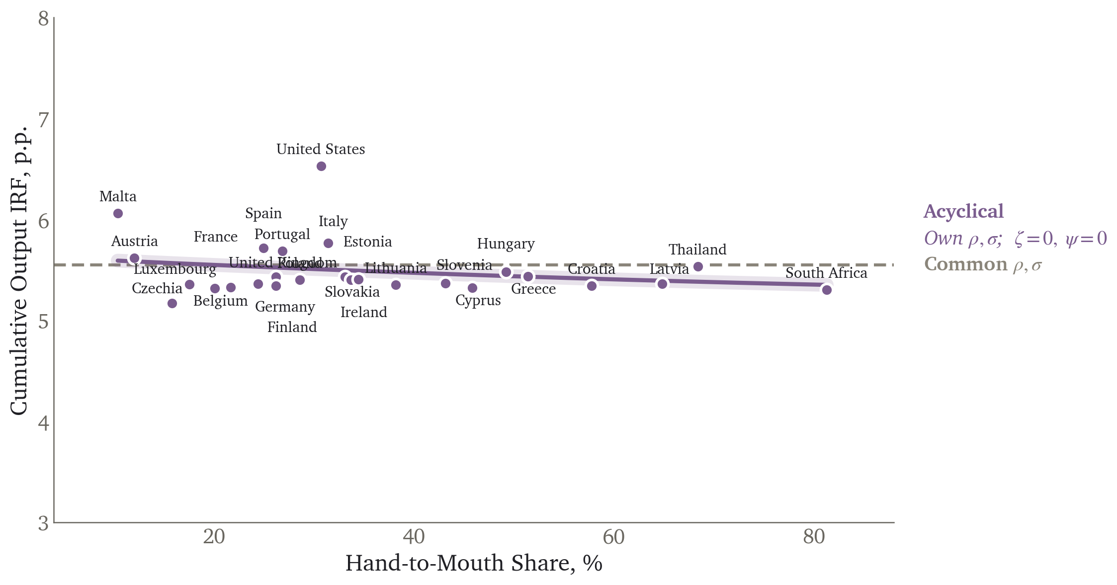
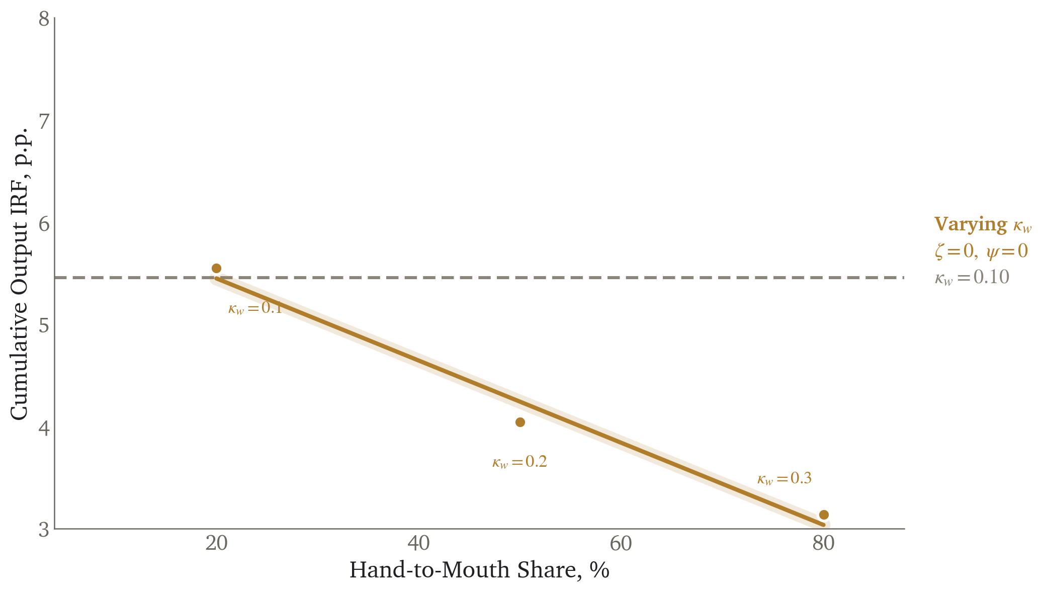
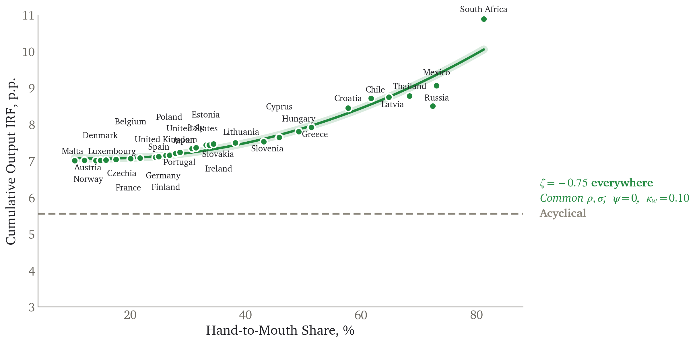
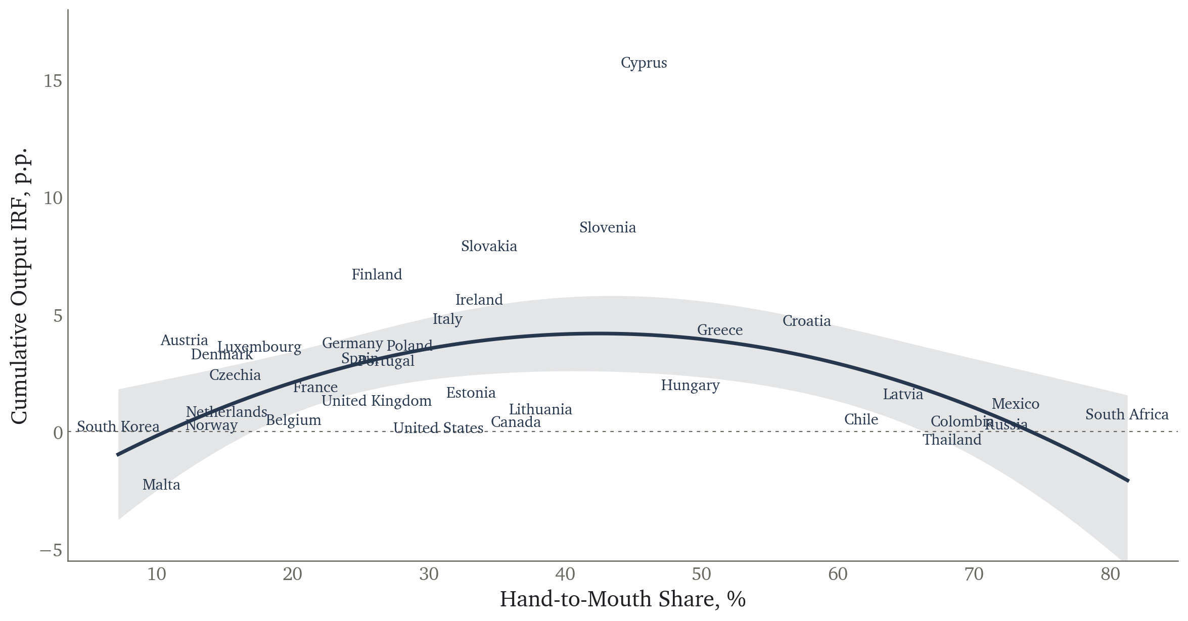
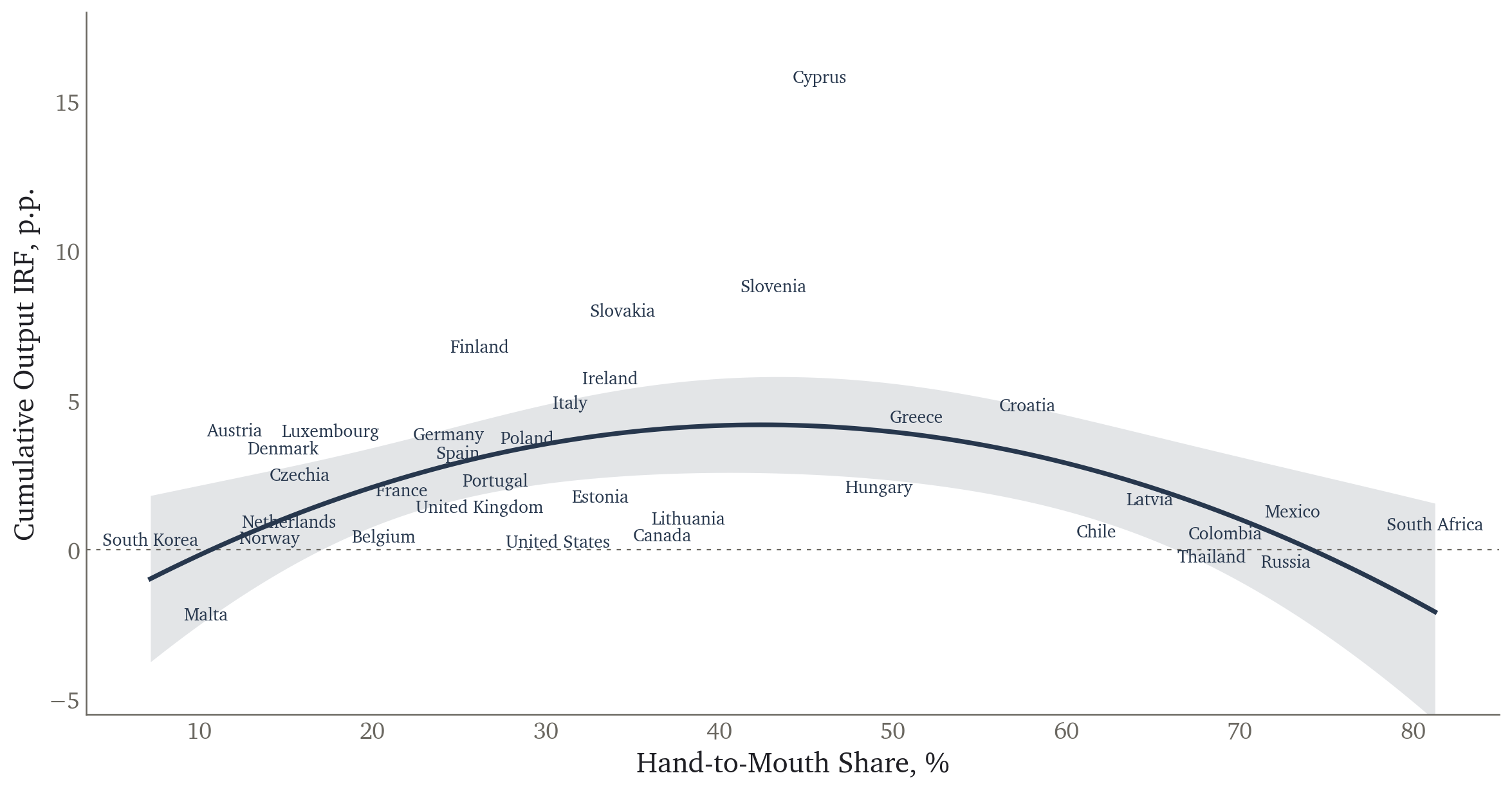
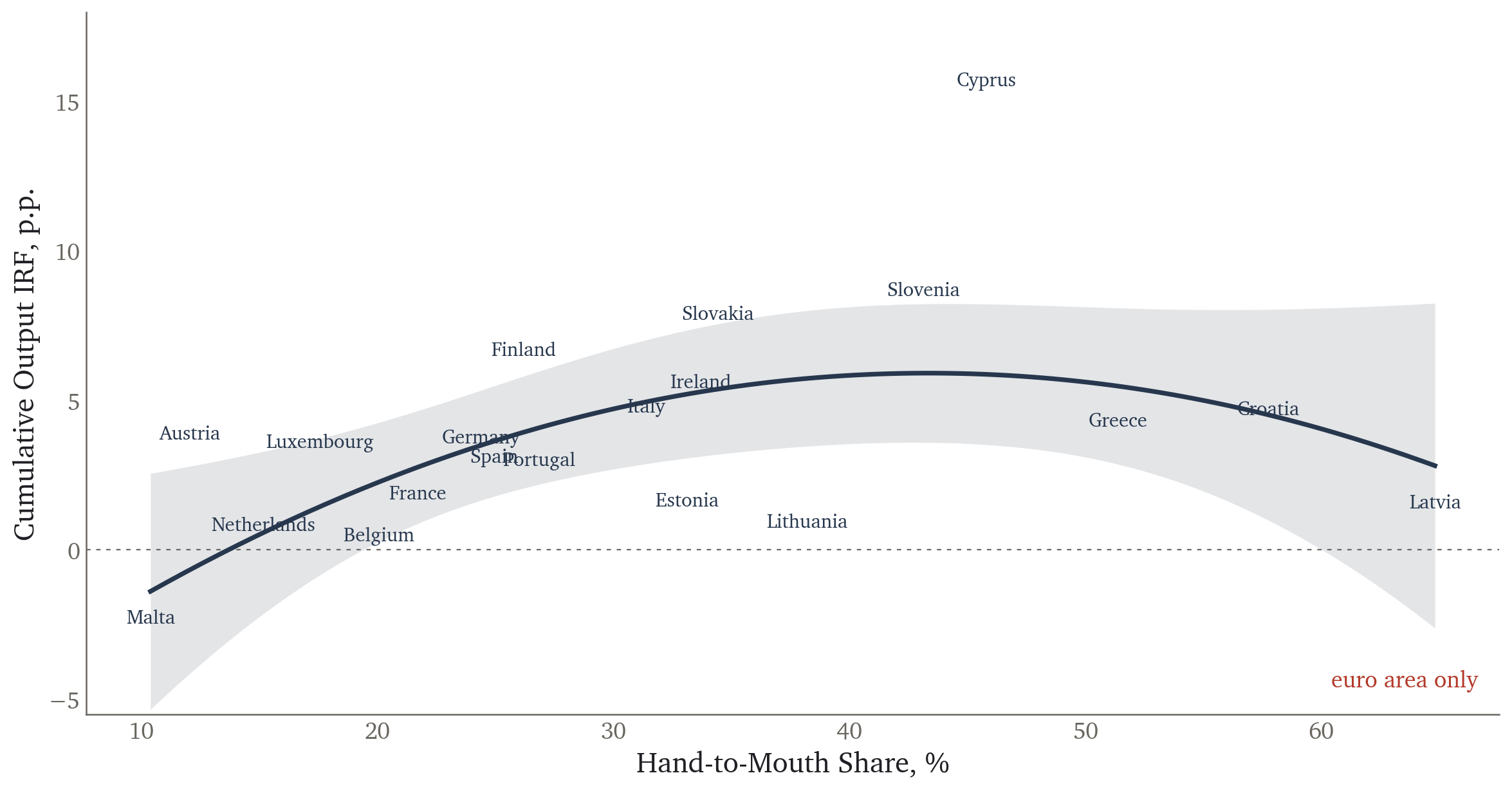
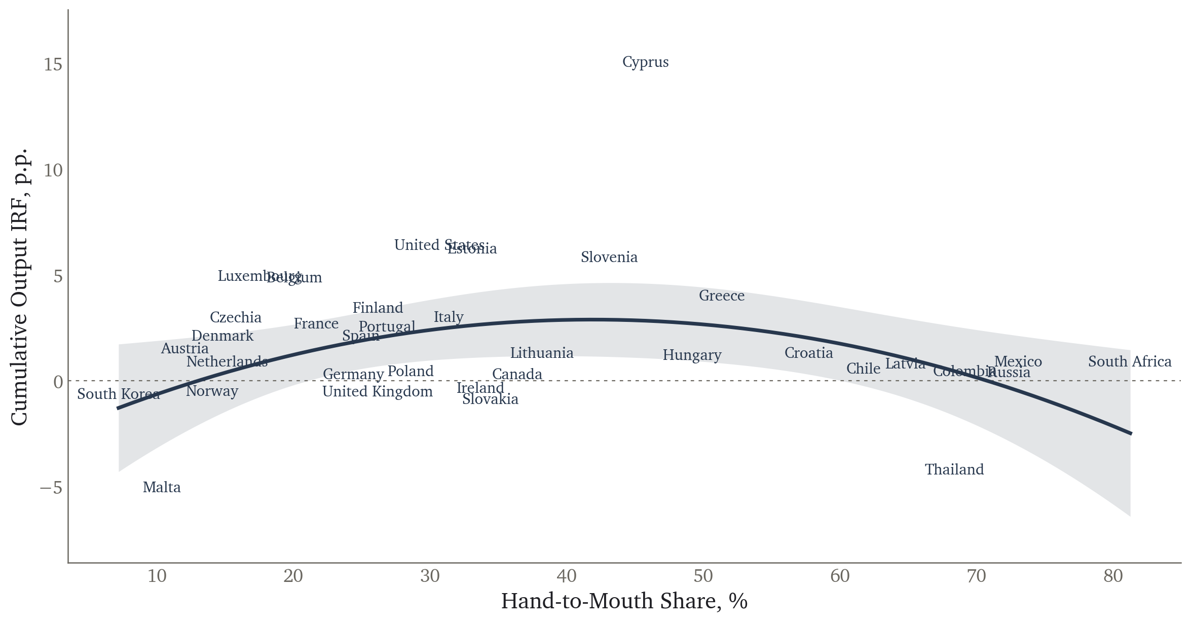
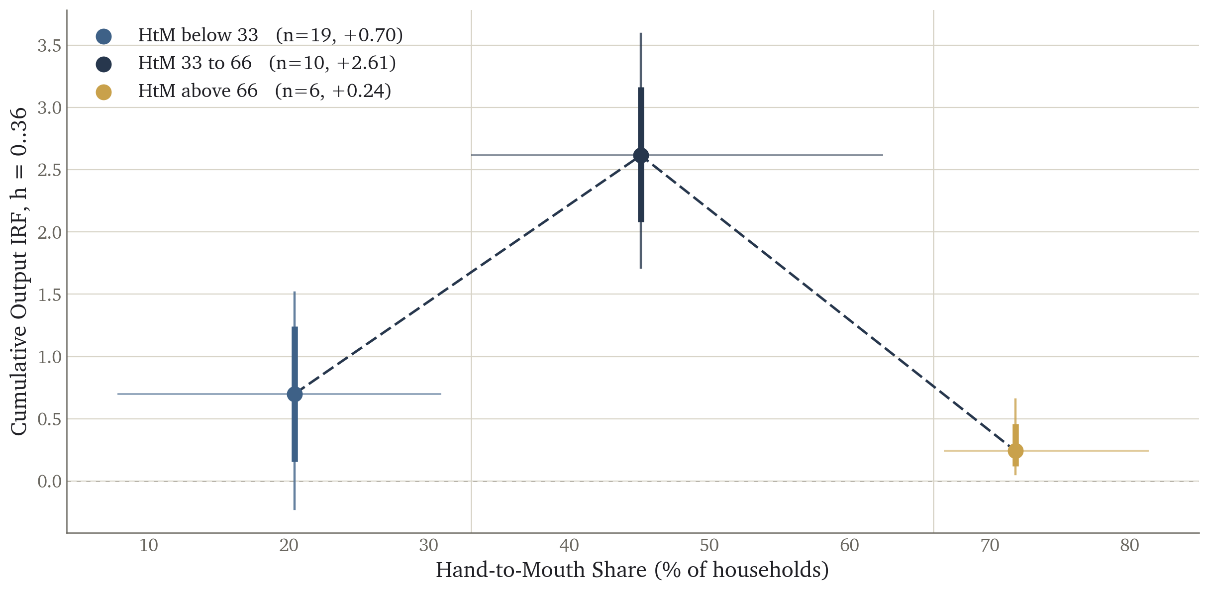
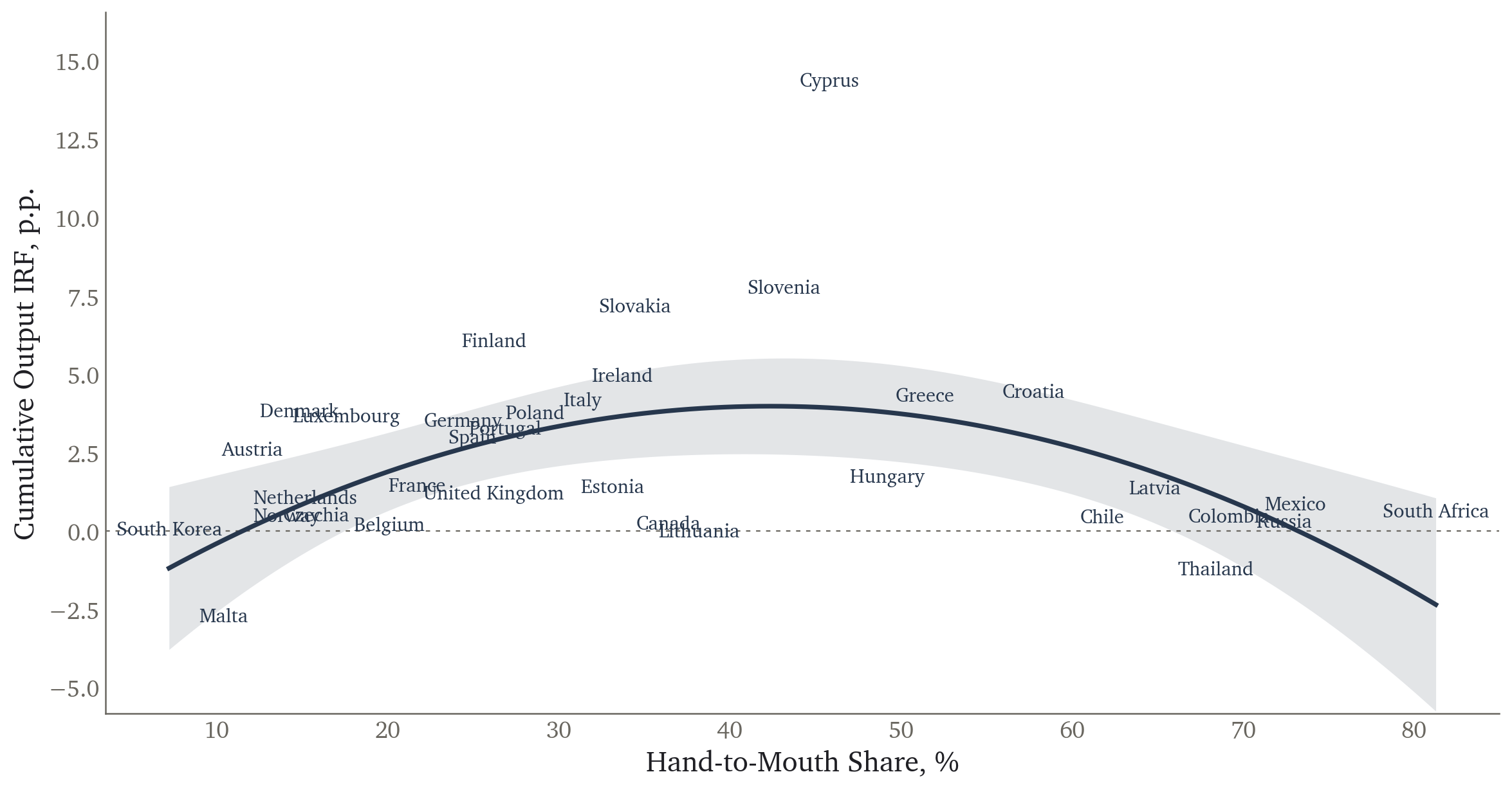
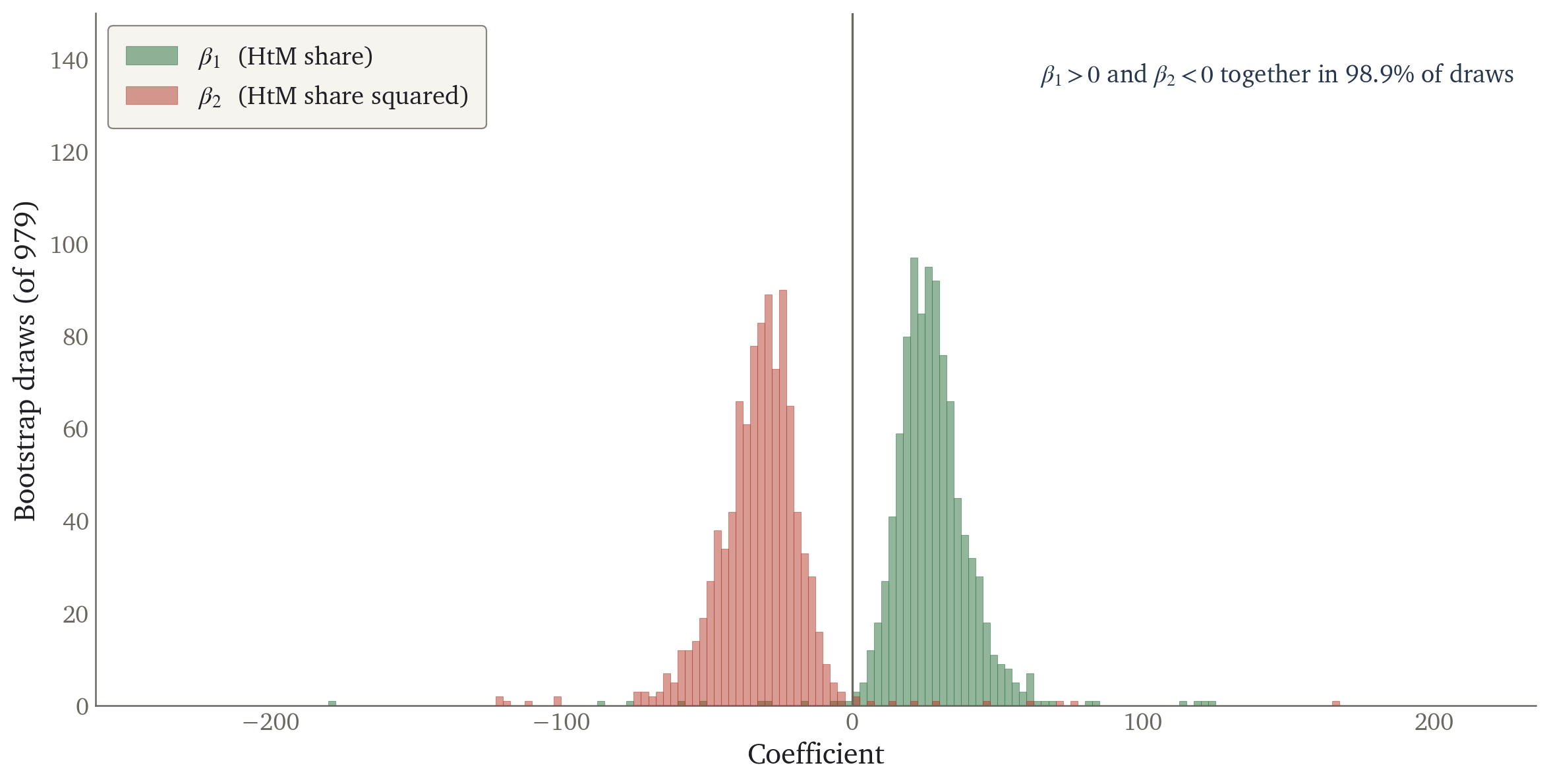
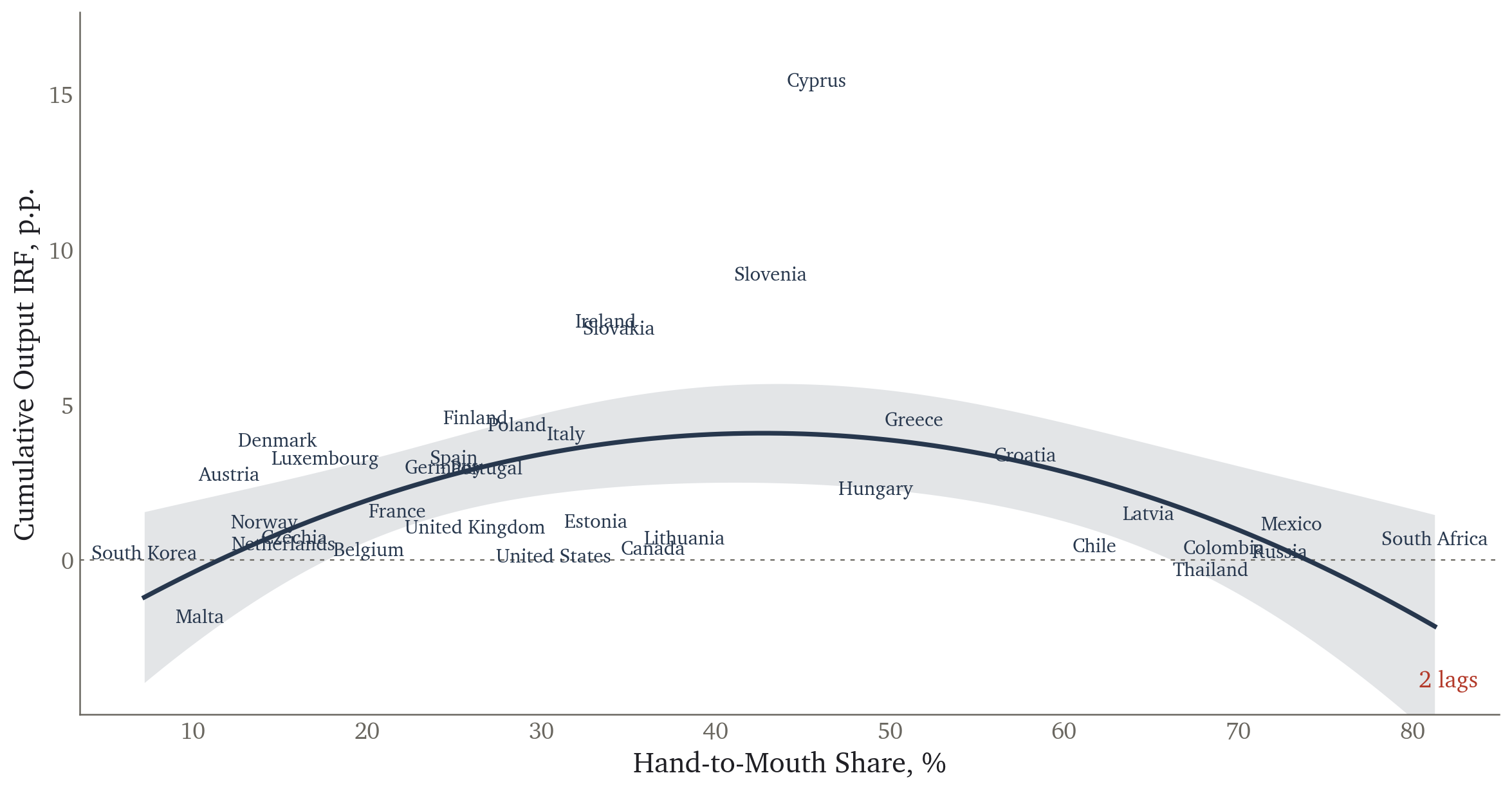
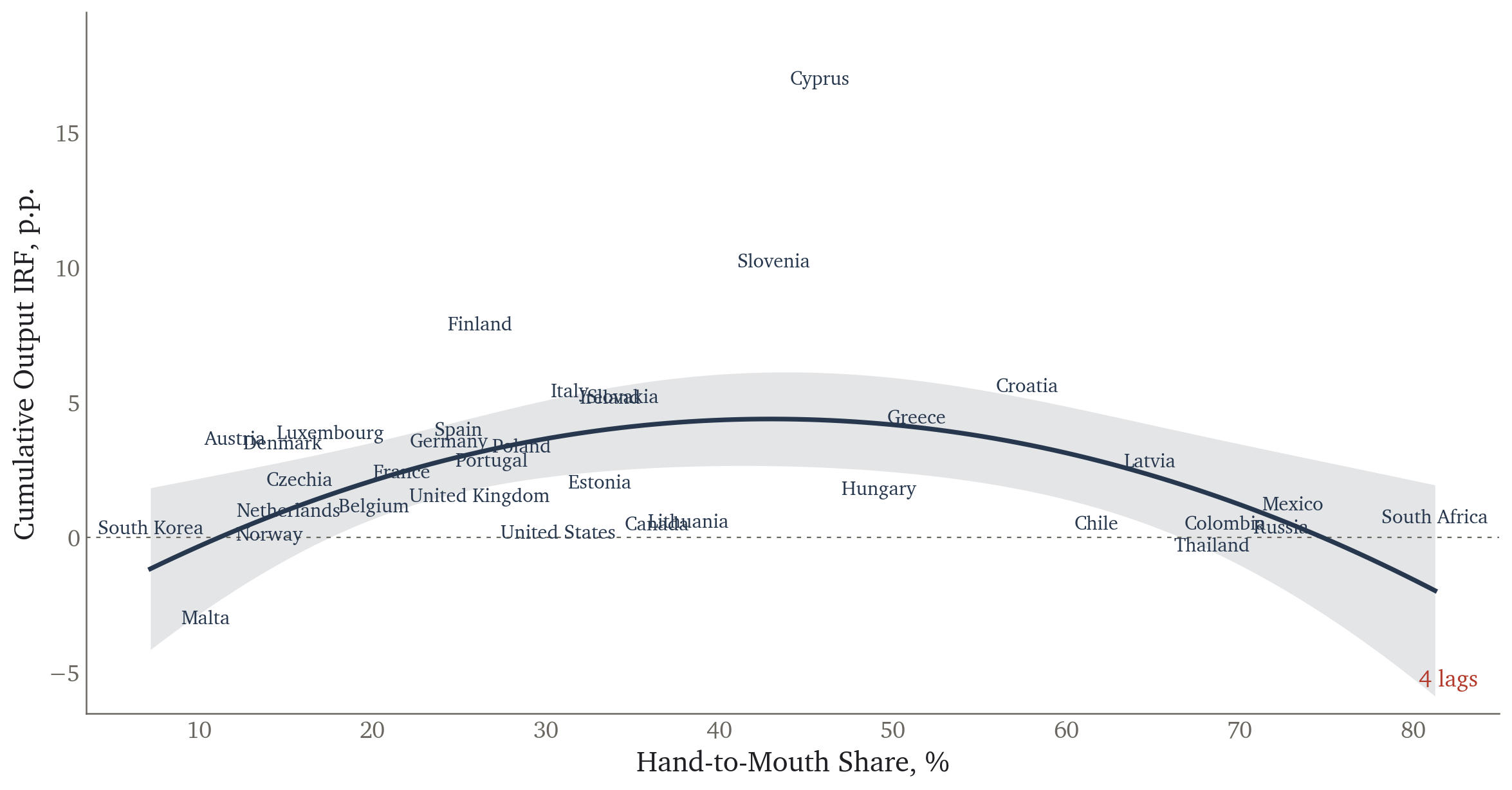
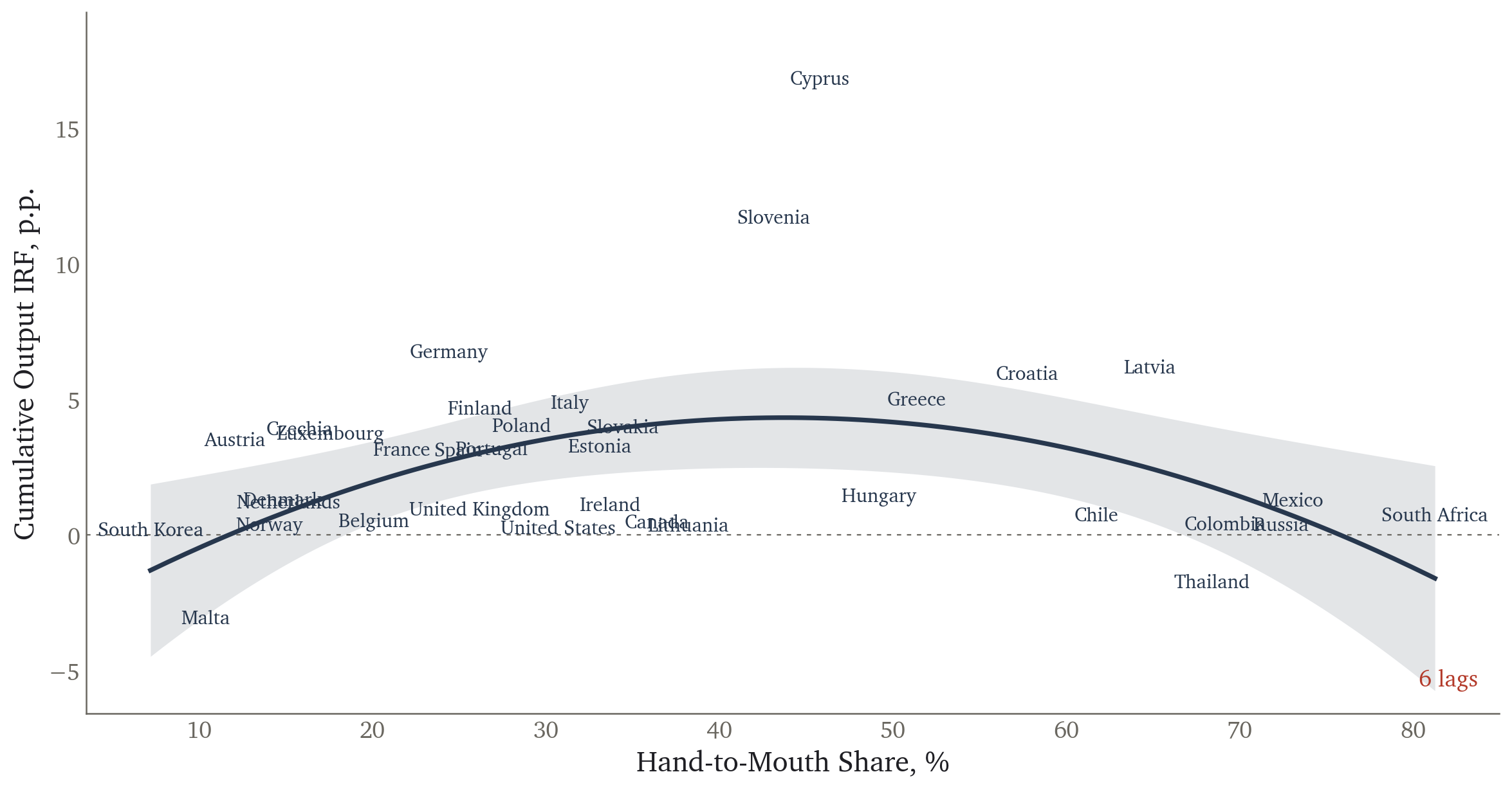
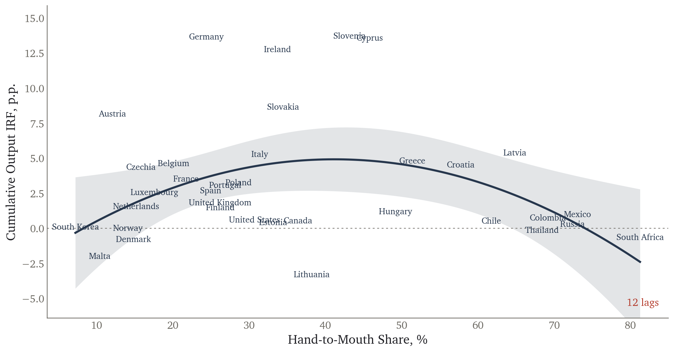
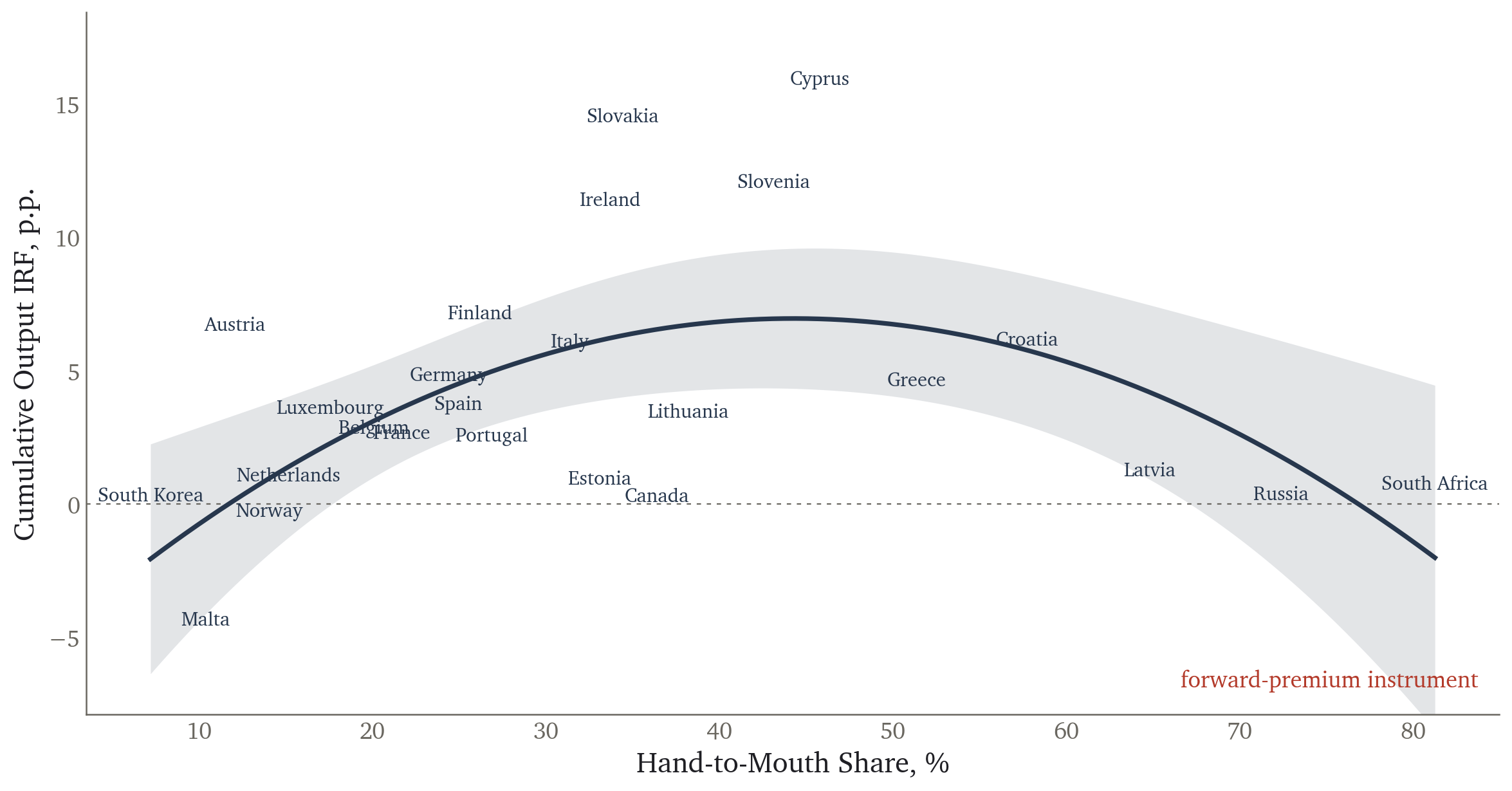
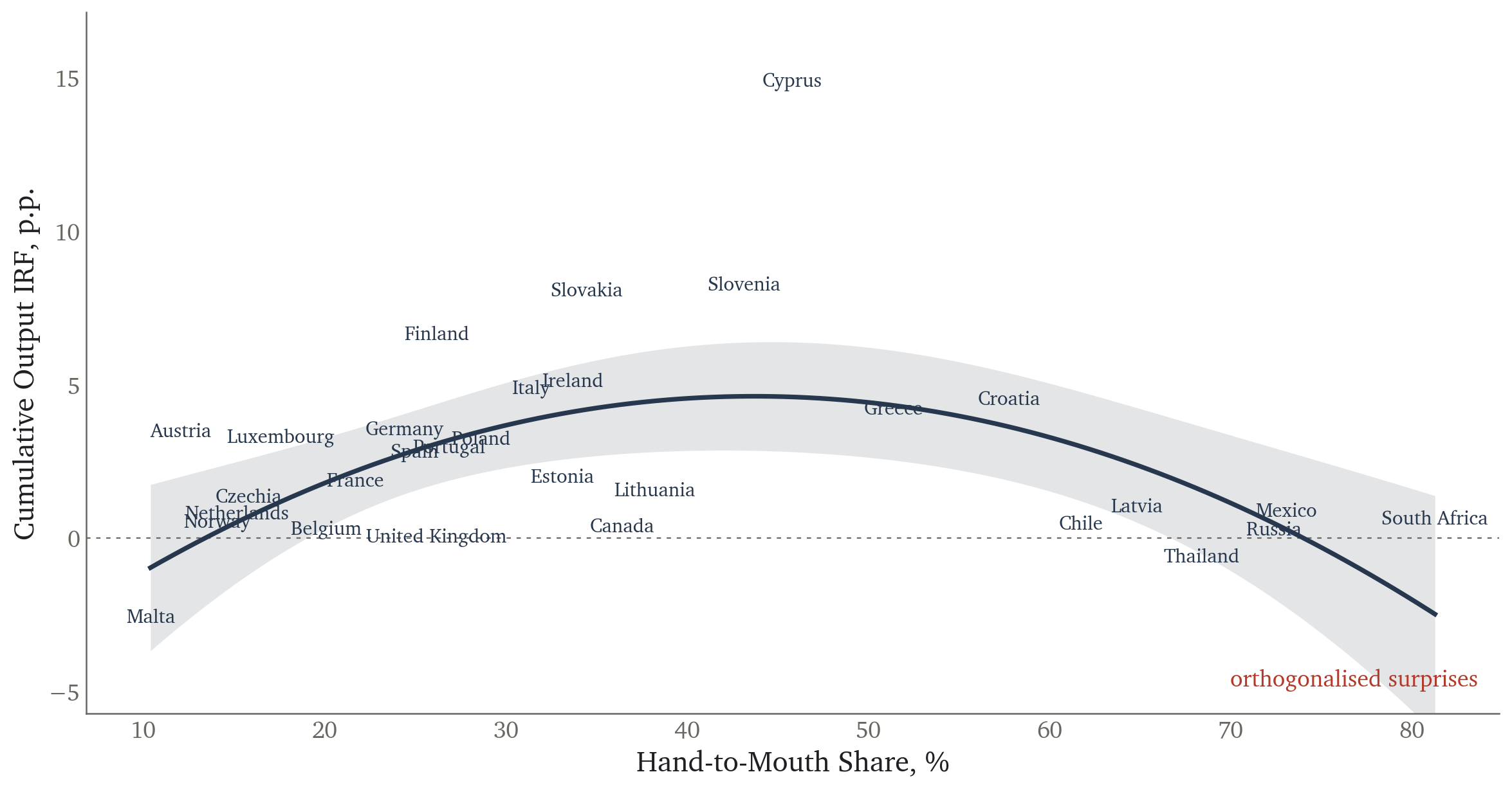
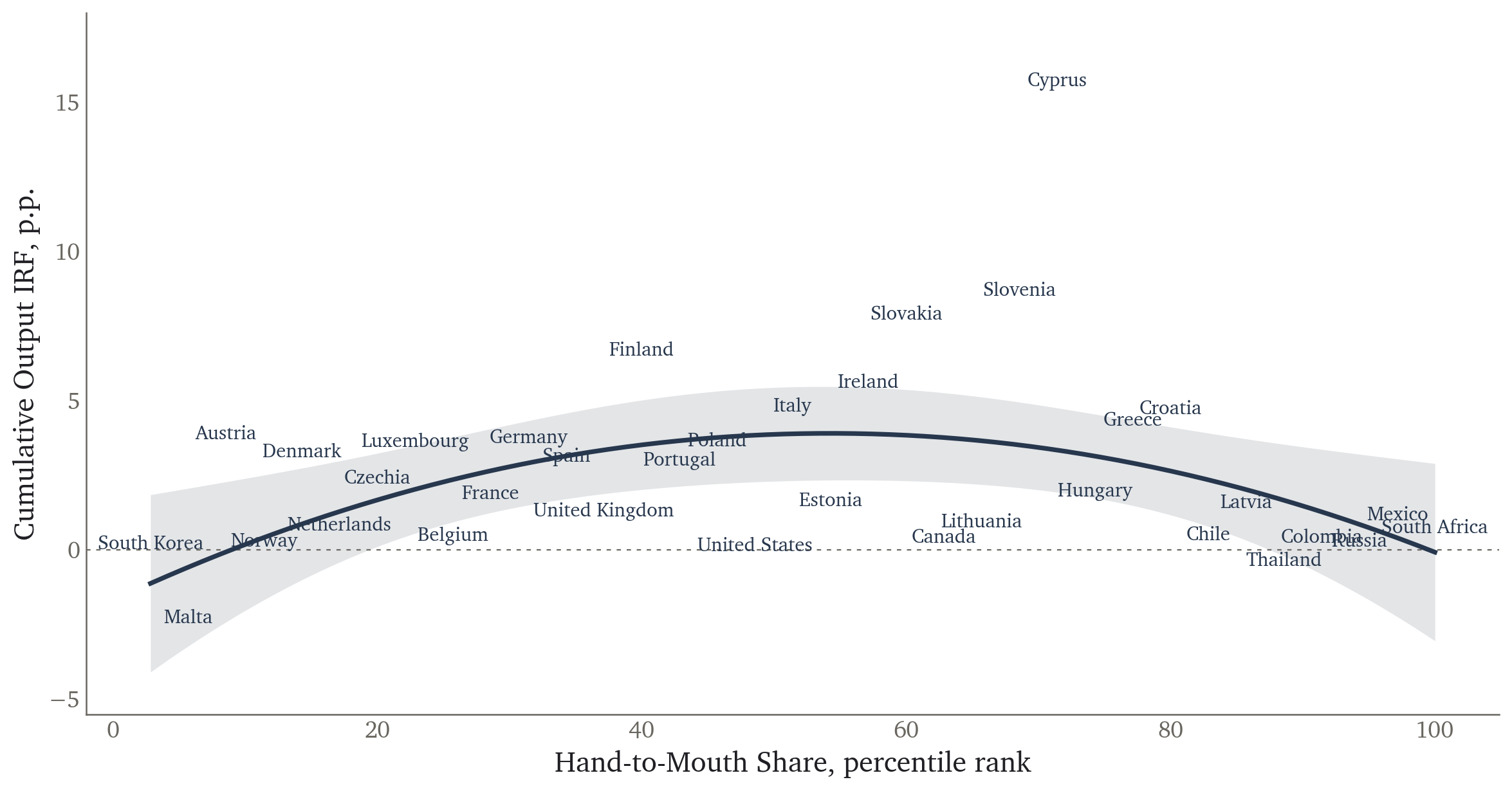
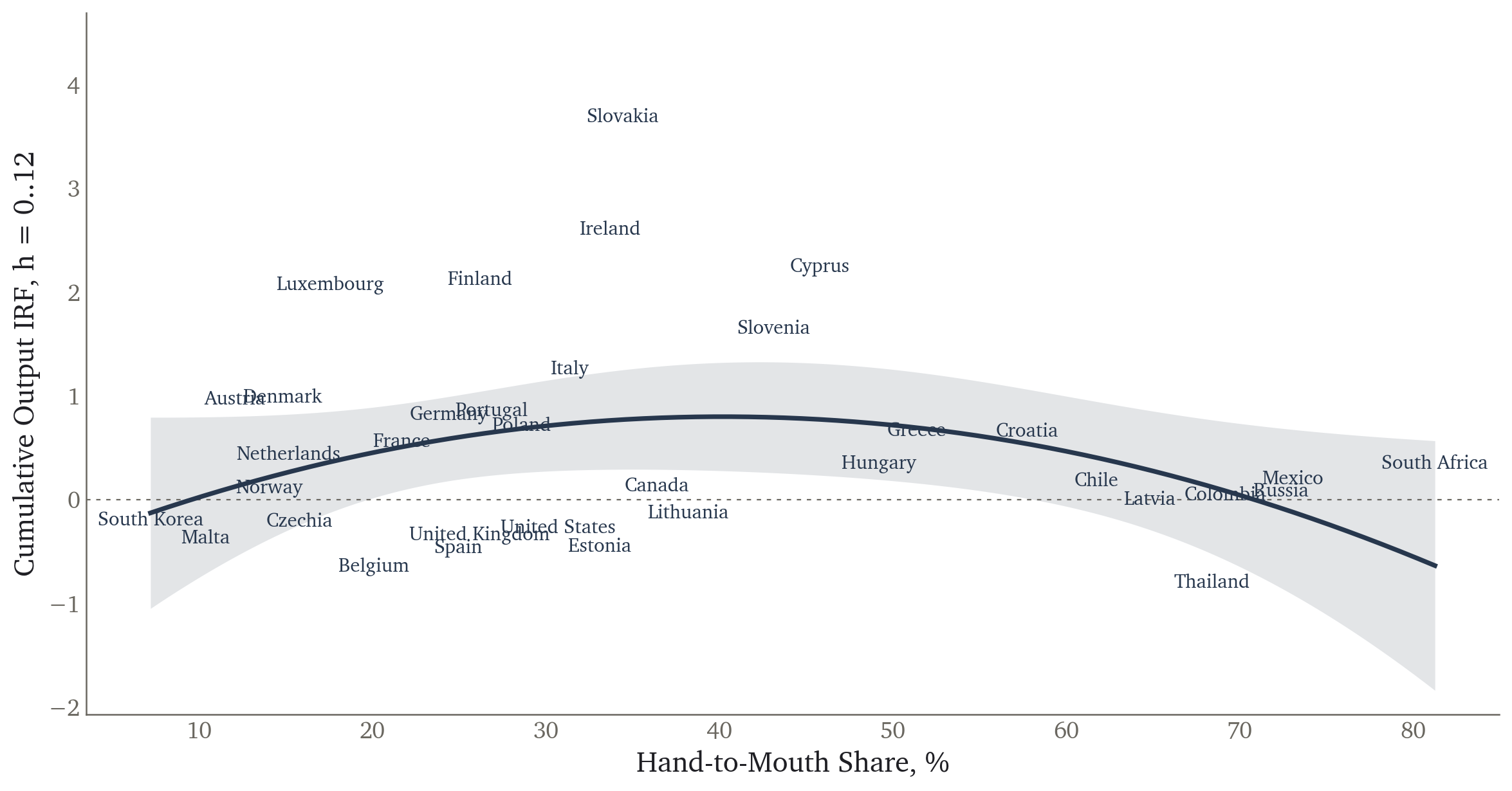
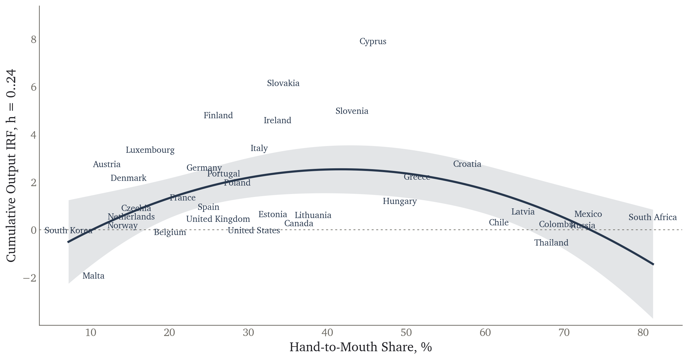
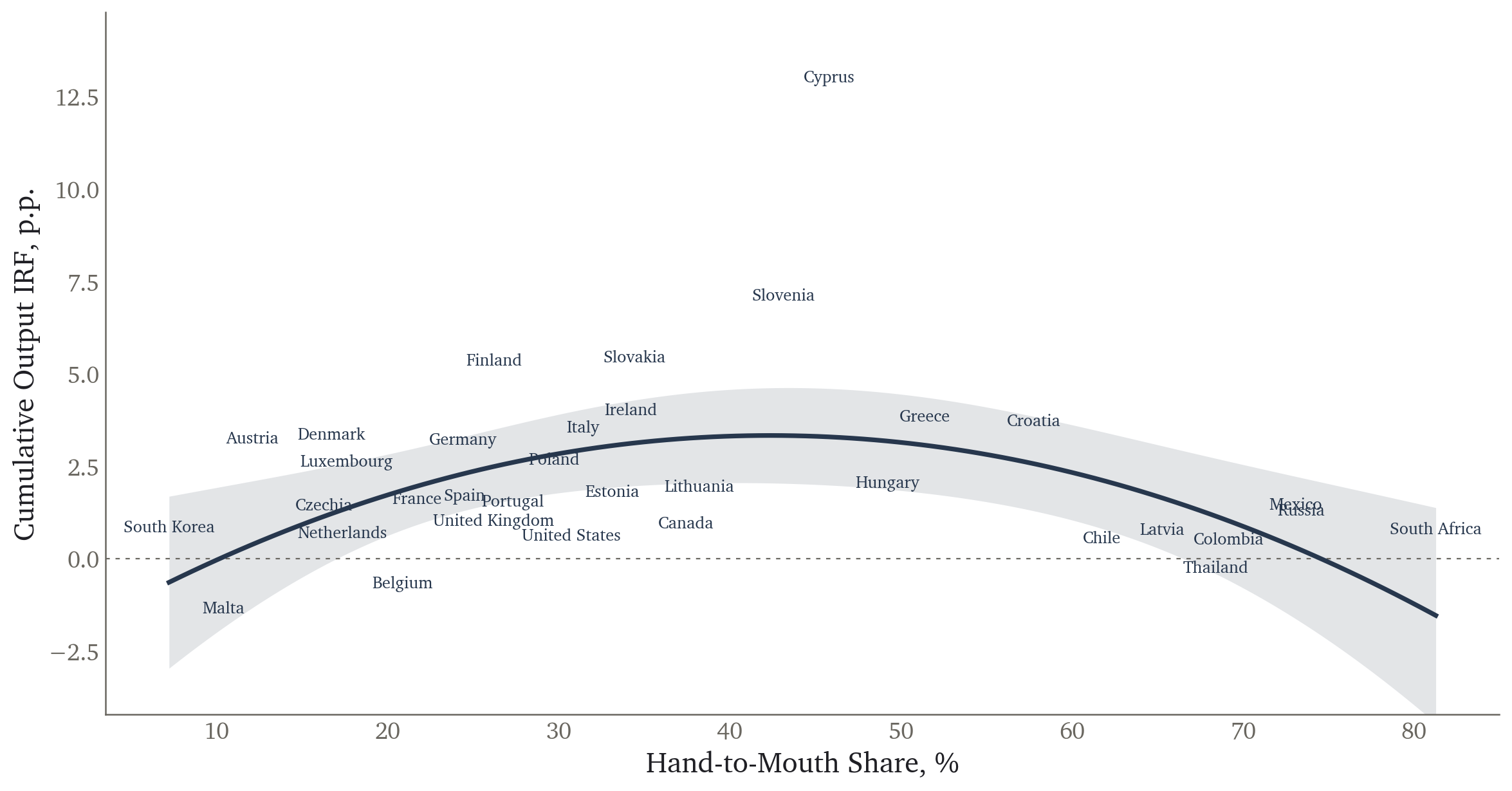
Output Responses and Hand-to-Mouth Shares
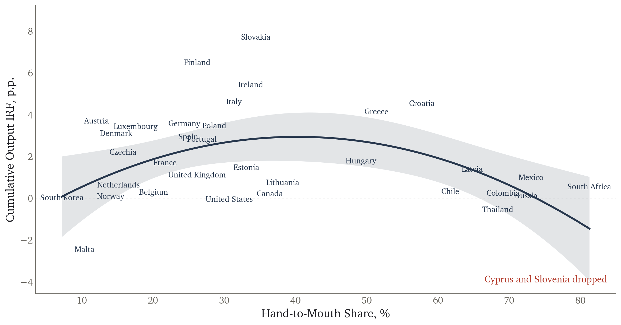
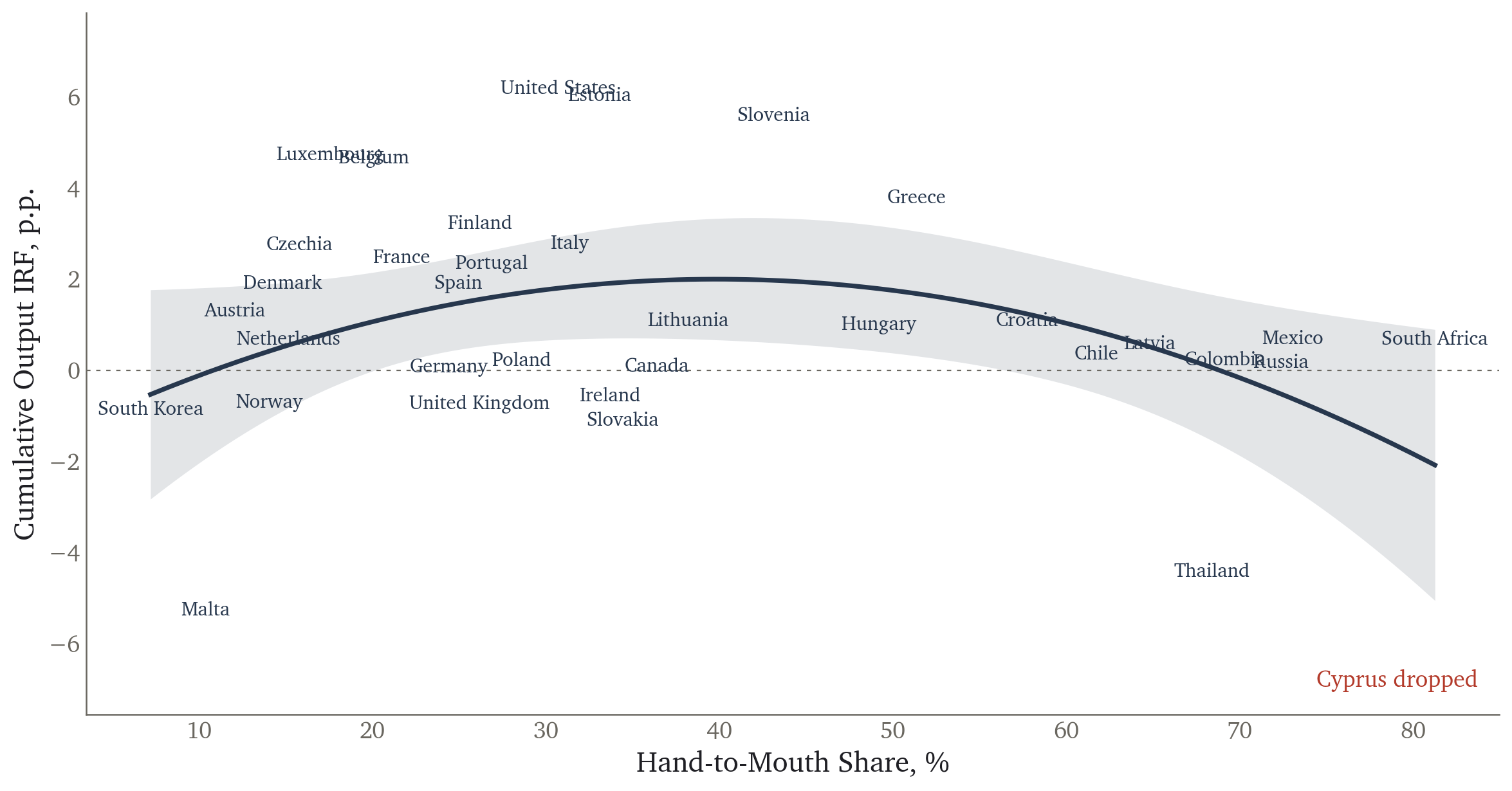
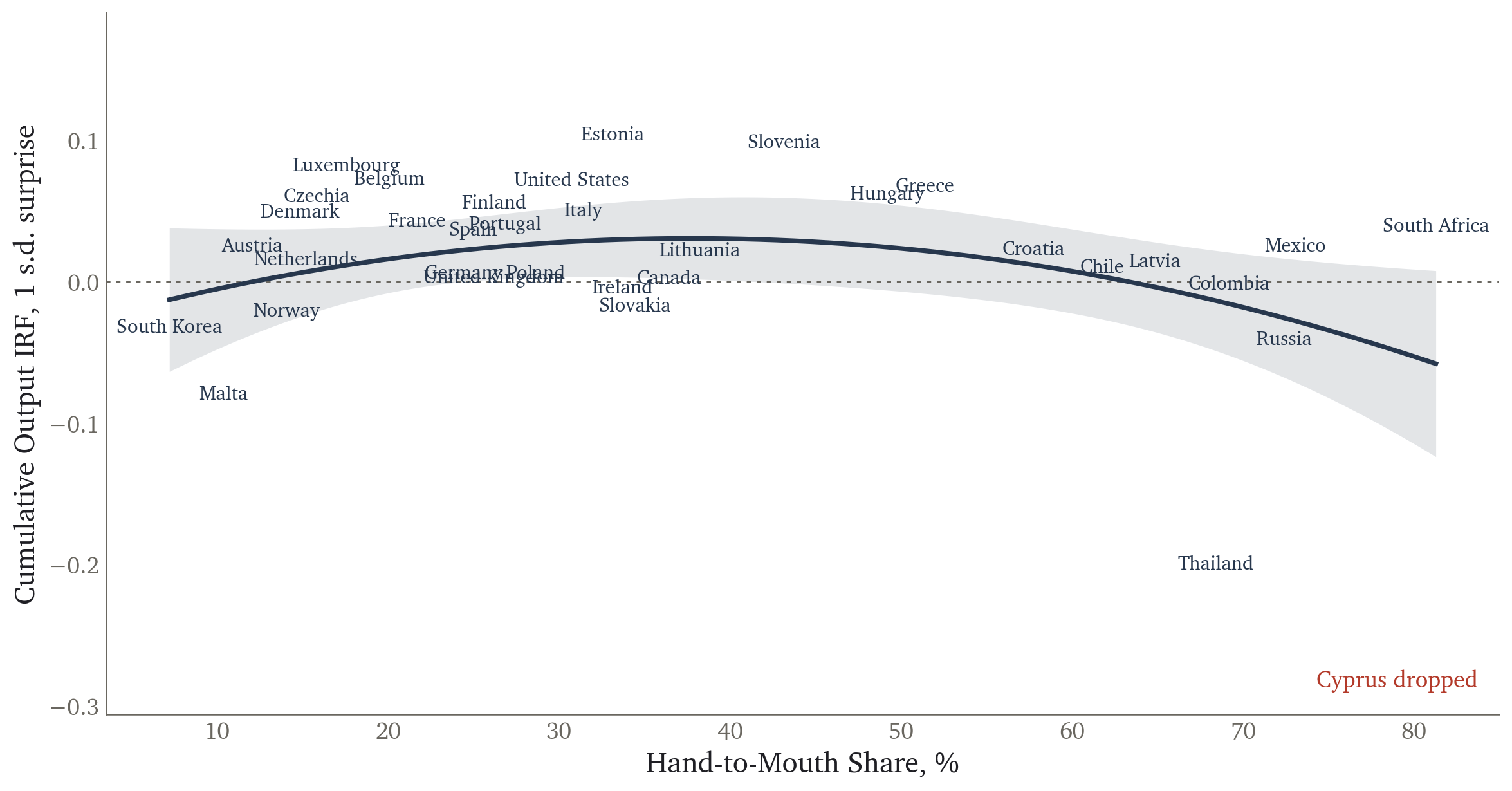
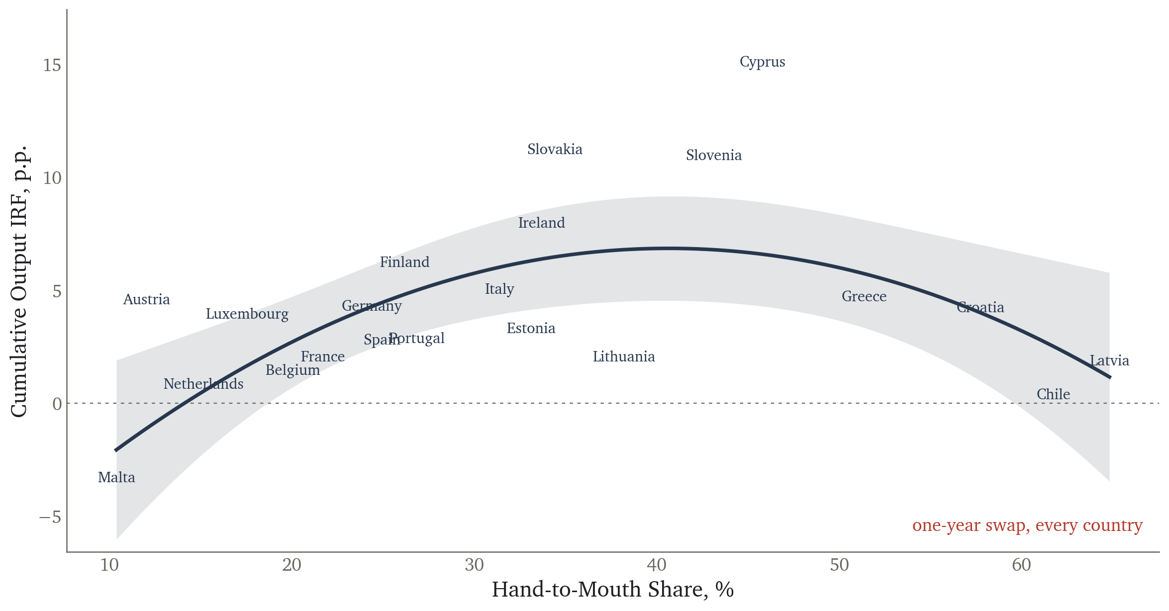
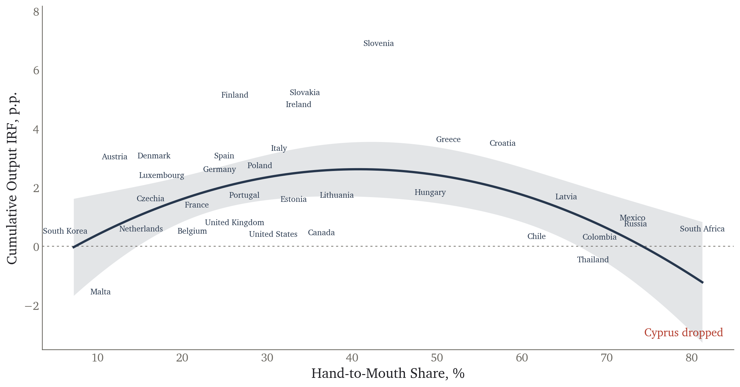
Output Responses and Hand-to-Mouth Shares Without Cyprus
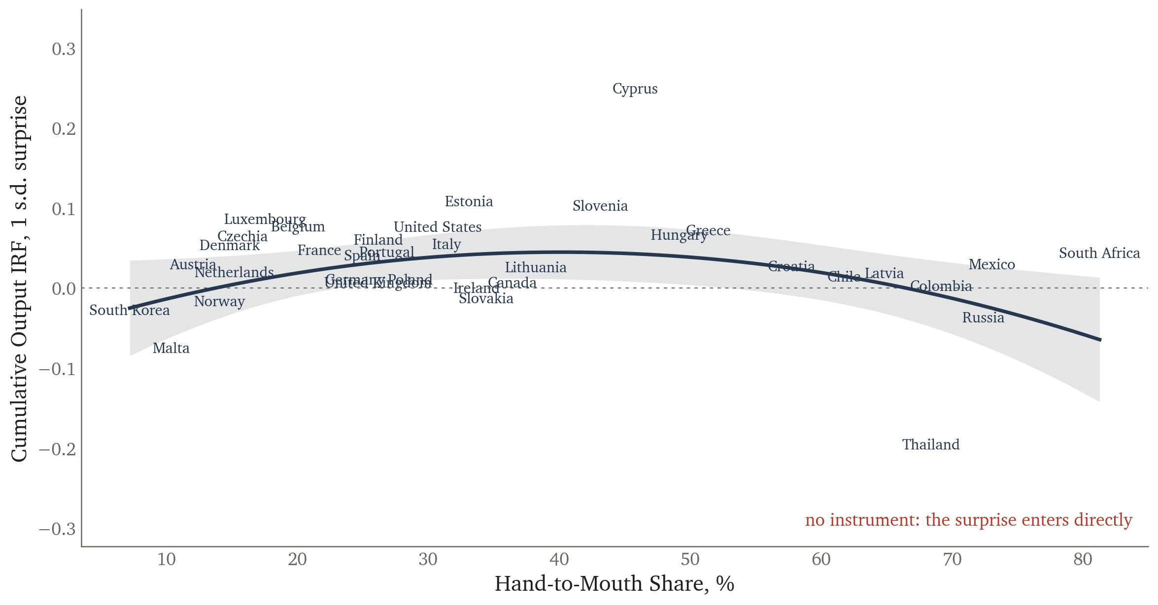
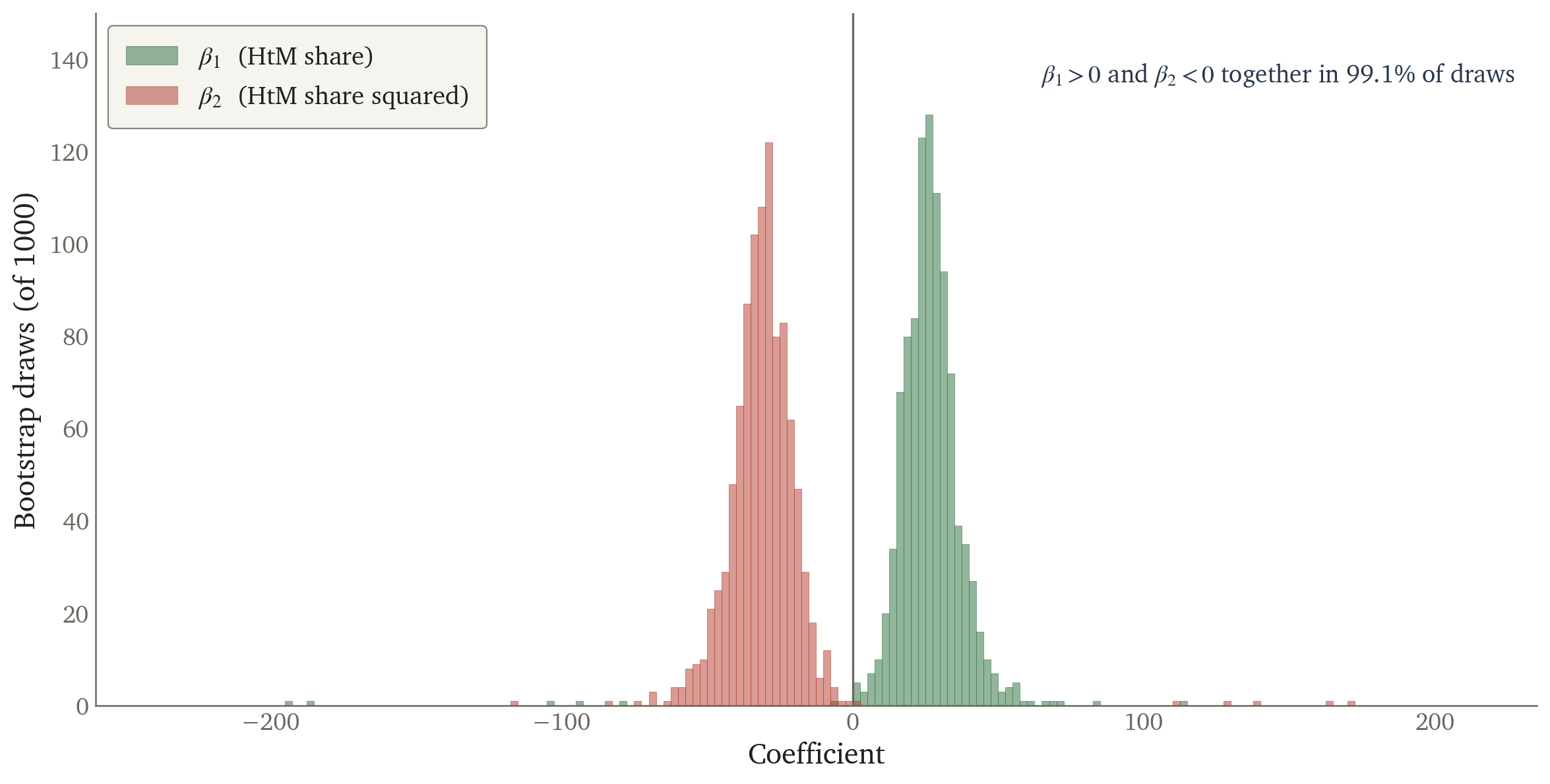
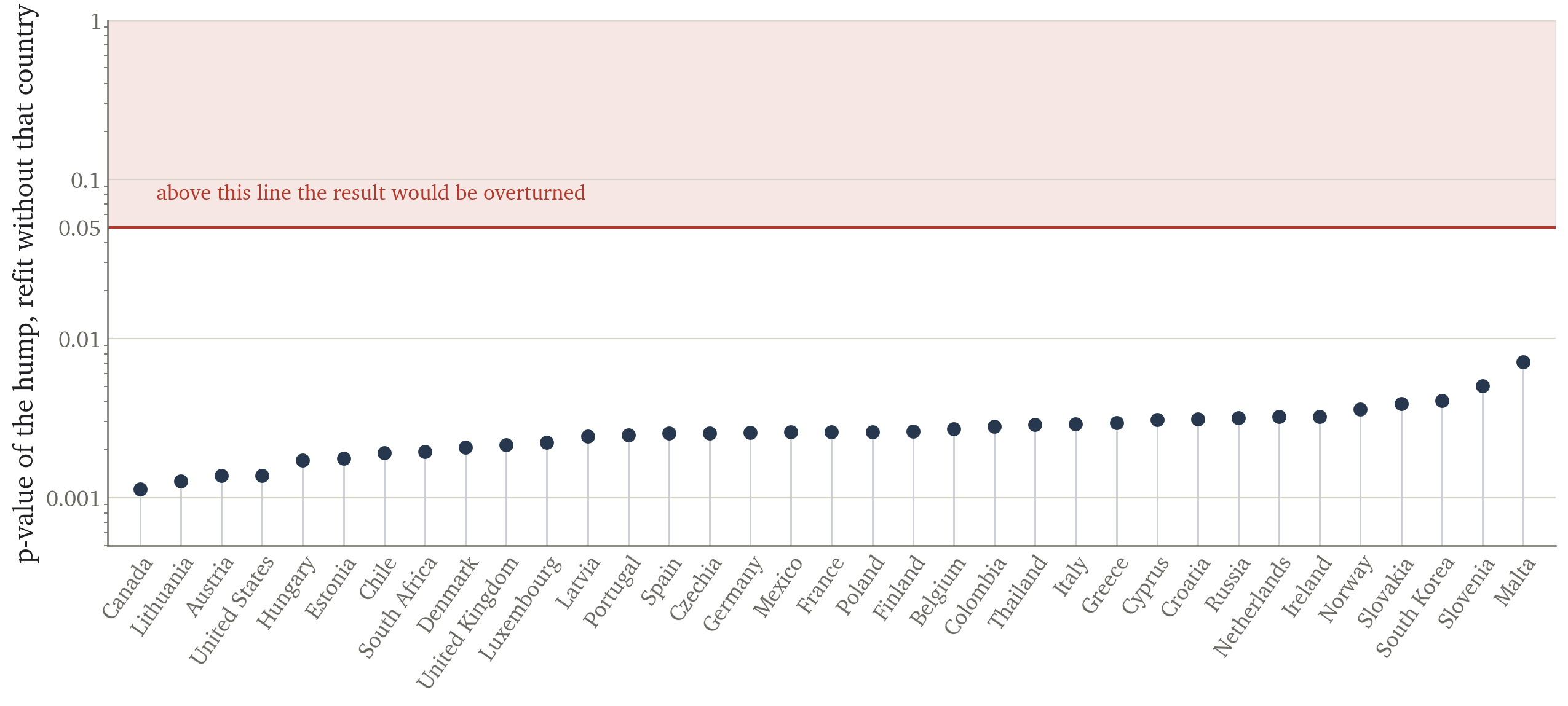
Output Responses and Hand-to-Mouth Shares Leave One Out
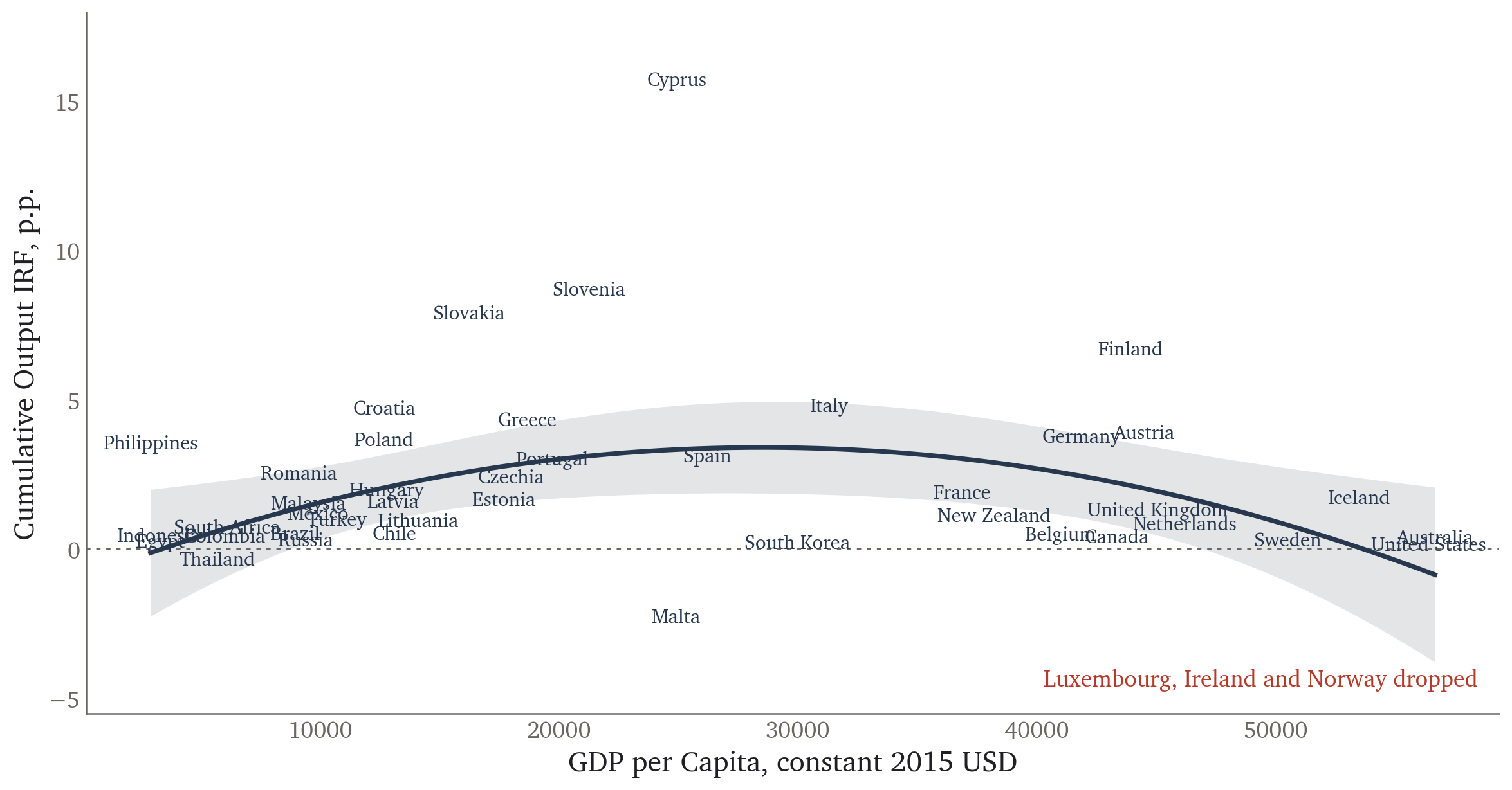
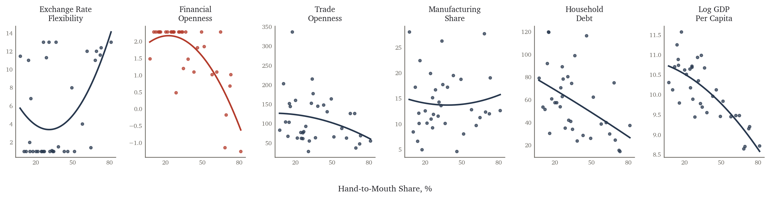
Output Responses and Hand-to-Mouth Shares Country Characteristics
Cumulative Output Response, p.p.
(1)
(2)
(3)
(4)
(5)
(6)
(7)
Hand-to-Mouth Share
Exchange Rate Flexibility
Financial Openness
Trade Openness
Manufacturing Share
Household Debt
Log GDP Per Capita
HtM
0.3523***
0.2834**
0.3457**
0.3432***
0.3813***
0.3647***
0.3173**
(0.1136)
(0.1105)
(0.1266)
(0.1162)
(0.1174)
(0.1139)
(0.1241)
HtM2
-0.0042***
-0.0030**
-0.0043**
-0.0040***
-0.0044***
-0.0043***
-0.0032*
(0.0013)
(0.0013)
(0.0016)
(0.0013)
(0.0013)
(0.0013)
(0.0016)
X
-1.3854
-1.1774
0.7542
-0.4009
0.1076
0.9127
(0.8625)
(1.1359)
(0.7152)
(0.5921)
(0.6901)
(0.9293)
X2
0.0530
-0.4225
-0.1758
0.5045
0.5611
-0.5444
(1.3227)
(0.4767)
(0.3075)
(0.4188)
(0.4958)
(0.5901)
R2
0.24
0.37
0.28
0.27
0.28
0.30
0.27
N
35
35
34
35
35
35
35
Output Responses and Hand-to-Mouth Shares Country Characteristics
Cumulative Output Response, p.p.
(1)
(2)
(3)
(4)
(5)
(6)
(7)
Hand-to-Mouth Share
Exchange Rate Flexibility
Financial Openness
Trade Openness
Manufacturing Share
Household Debt
Log GDP Per Capita
HtM
0.3523***
0.2834**
0.3457**
0.3432***
0.3813***
0.3647***
0.3173**
(0.1136)
(0.1105)
(0.1266)
(0.1162)
(0.1174)
(0.1139)
(0.1241)
HtM2
-0.0042***
-0.0030**
-0.0043**
-0.0040***
-0.0044***
-0.0043***
-0.0032*
(0.0013)
(0.0013)
(0.0016)
(0.0013)
(0.0013)
(0.0013)
(0.0016)
X
-1.3854
-1.1774
0.7542
-0.4009
0.1076
0.9127
(0.8625)
(1.1359)
(0.7152)
(0.5921)
(0.6901)
(0.9293)
X2
0.0530
-0.4225
-0.1758
0.5045
0.5611
-0.5444
(1.3227)
(0.4767)
(0.3075)
(0.4188)
(0.4958)
(0.5901)
R2
0.24
0.37
0.28
0.27
0.28
0.30
0.27
N
35
35
34
35
35
35
35
Output Responses and Hand-to-Mouth Shares Robustness
Assets, liabilities, income, consumption and demographics for 35 countries, yearly, circa 2017
Canada: Survey of Financial Security (SFS) · Chile: Encuesta Financiera de Hogares (EFH) · Colombia: Encuesta de Carga Financiera y Educación Financiera (IEFIC) · Denmark: Wealth and other Administrative Registers · European Union: Household Finance and Consumption Survey (HFCS) · Mexico: Encuesta Nacional sobre las Finanzas de los Hogares (ENFIH) · Norway: Household Wealth Statistics · Russia: Russia Longitudinal Monitoring Survey (RLMS‑HSE) · South Africa: National Income Dynamics Study (NIDS) · South Korea: Survey of Household Finances and Living Conditions (SFLC) · Thailand: Townsend Thai Survey (TTS) · United Kingdom: Wealth and Assets Survey (WAS) · United States: Survey of Consumer Finances (SCF)
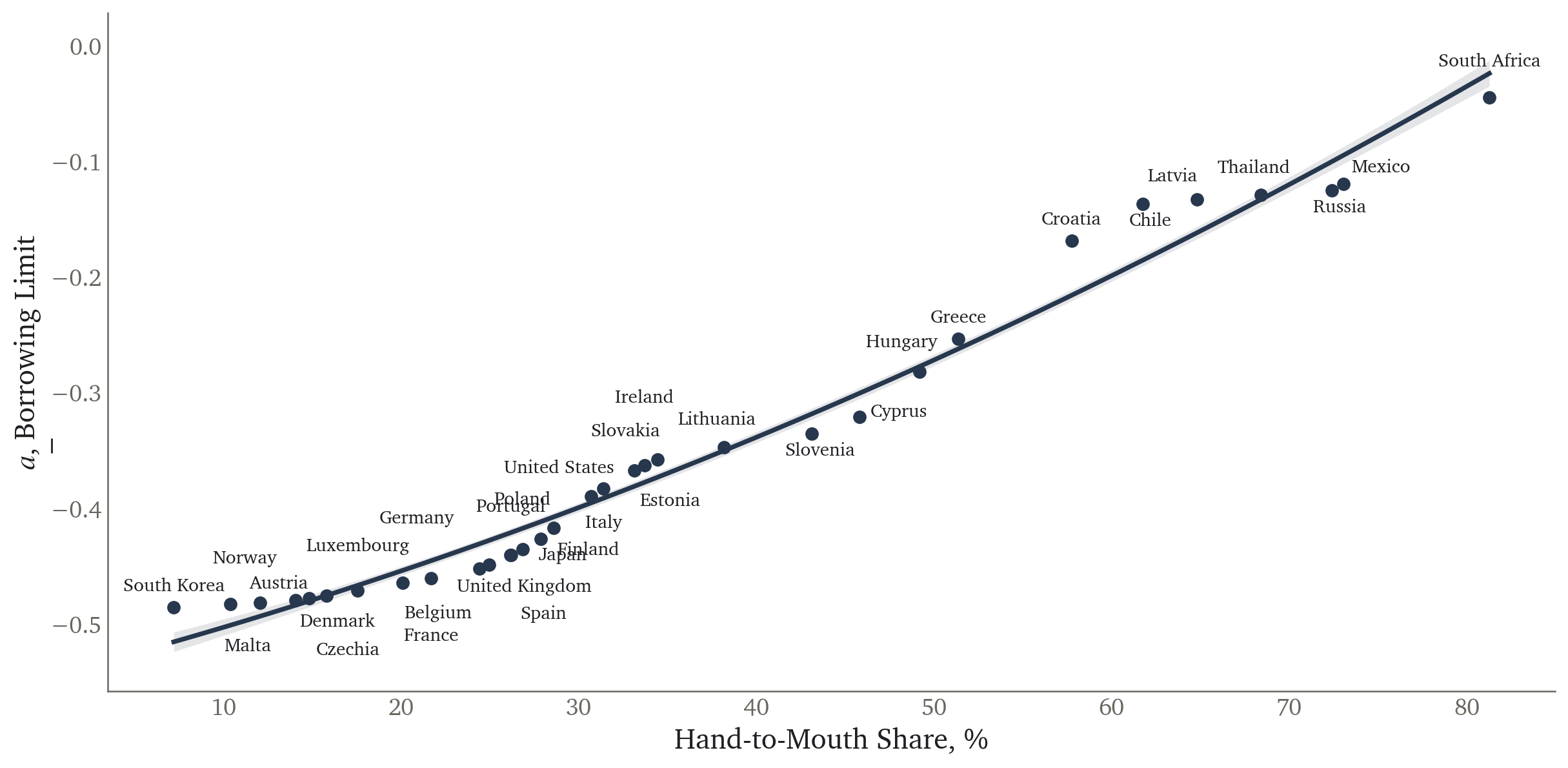
1. Borrowing Limit $\underline{a}$ Across Countries
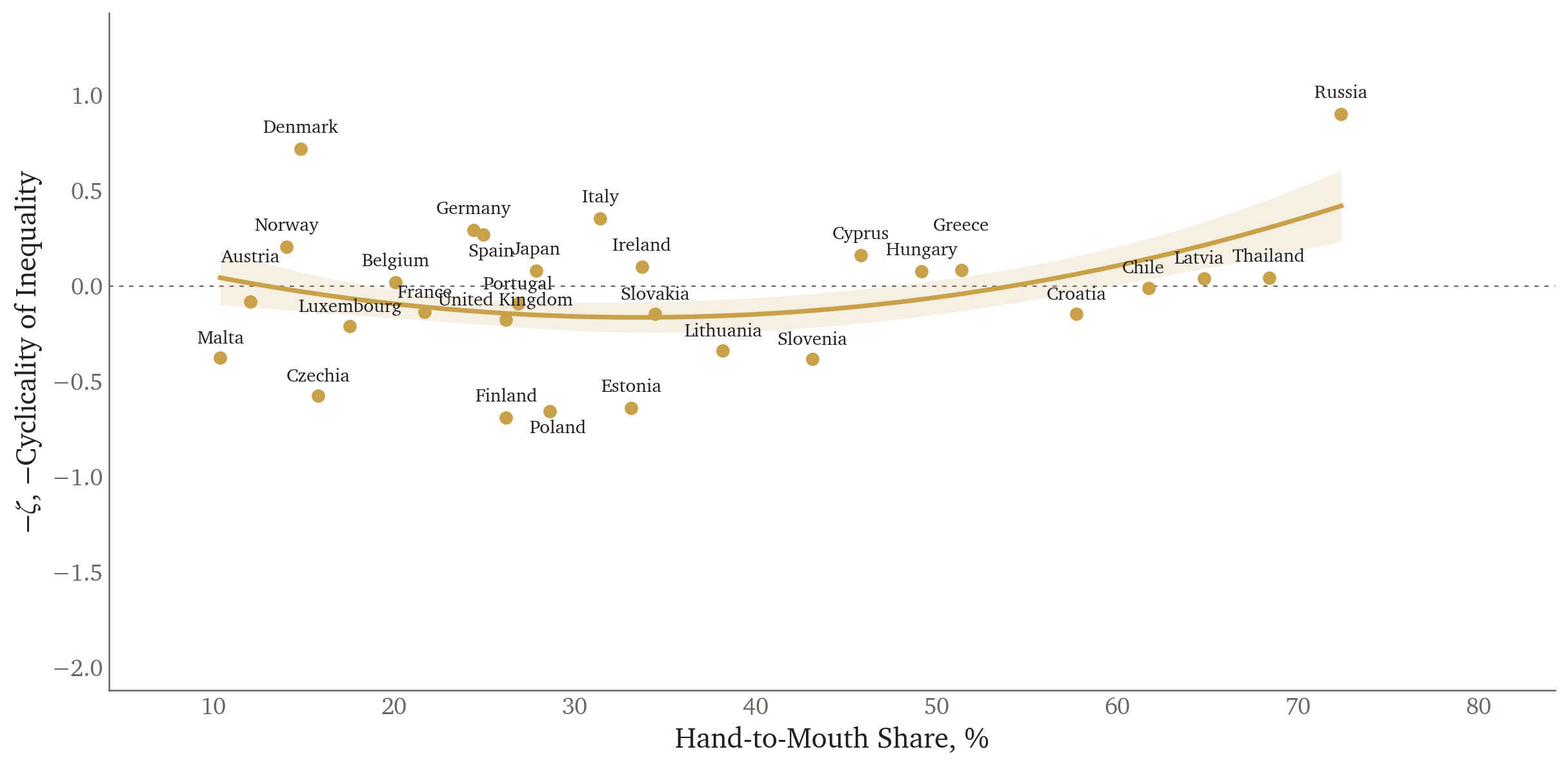
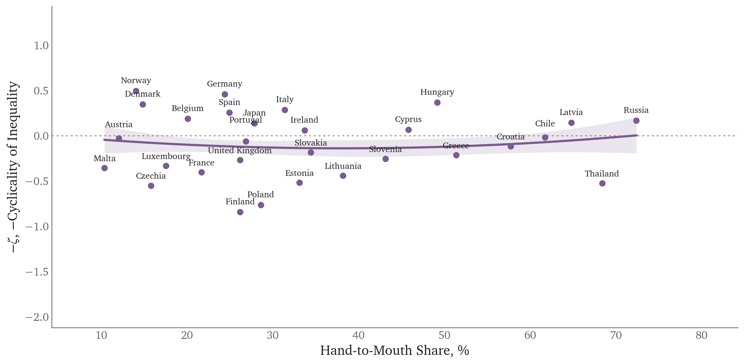
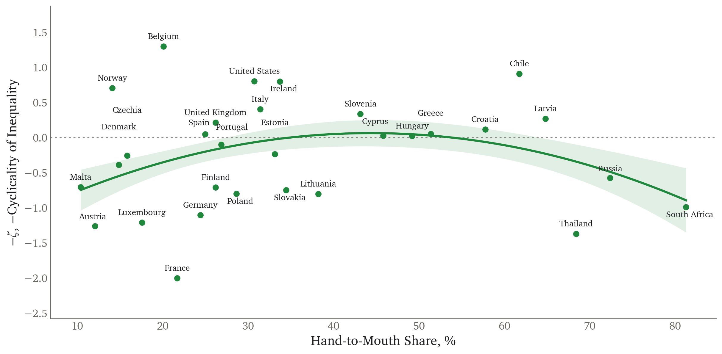
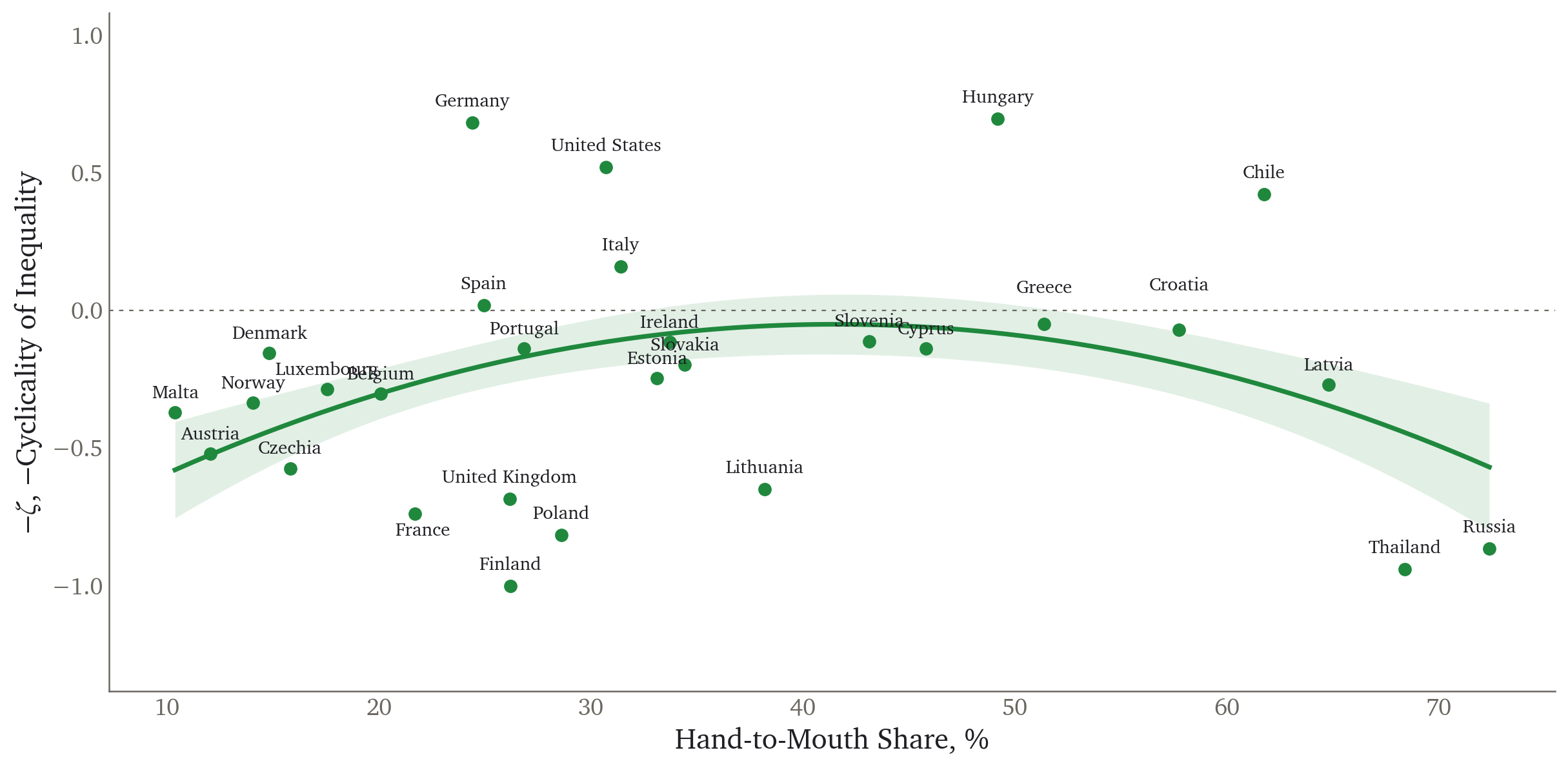
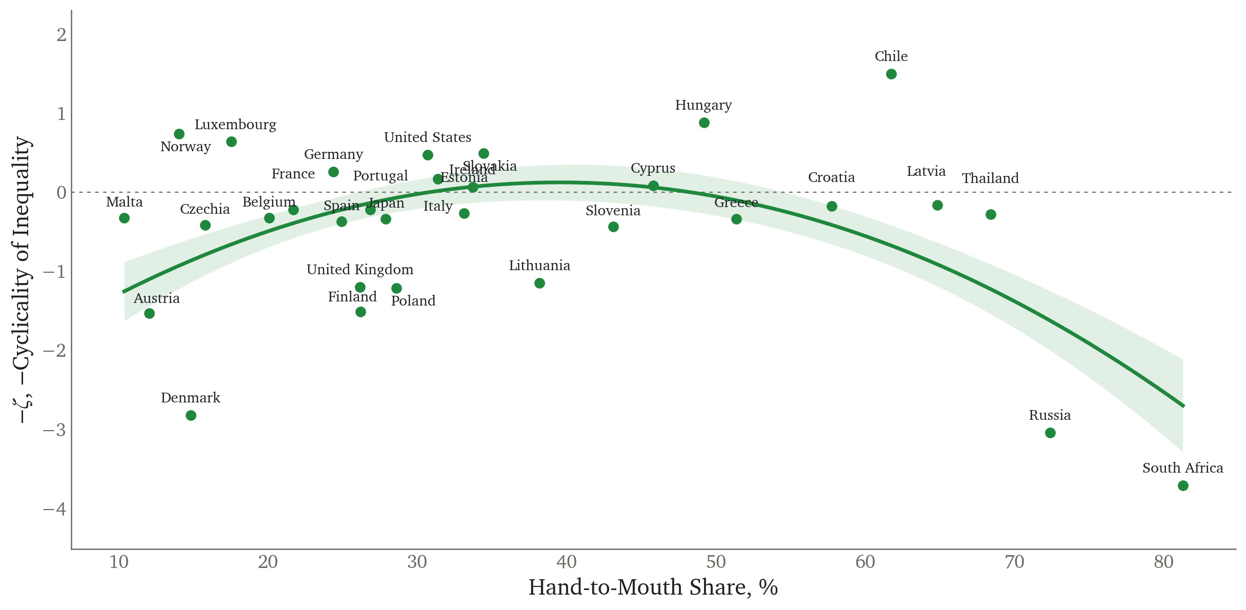
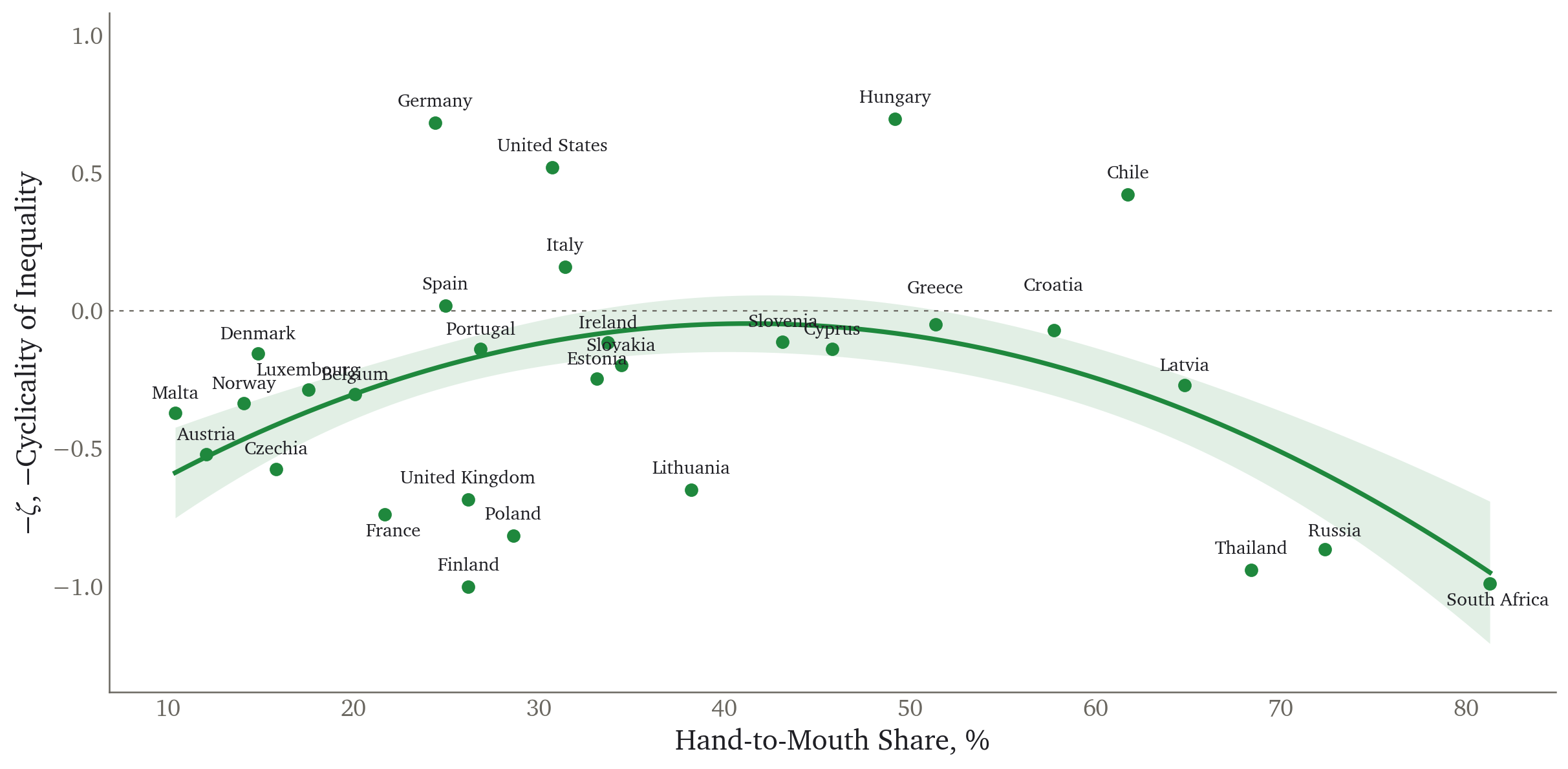
2. Cyclicality of Inequality $\zeta$ Calibration
Labour allocation rule$\displaystyle n_{it}(Y_t) \;=\; Y_t\, \frac{e_{it}^{\,{\color{#1f883d}\zeta}\log Y_t}}{\mathbb{E}\!\left[e_i^{\,1+{\color{#1f883d}\zeta}\log Y_t}\right]}$
Two steps, following Auclert & Rognlie (2018)
Step 1: Worker $\beta$s by lagged total income $y_{i,t-1}$ quintiles (Guvenen, Schulhofer-Wohl, Song & Yogo, 2017)
Labour and disposable income for 30 countries, yearly, circa 2005–2024
European Union: Statistics on Income and Living Conditions (EU‑SILC) · Italy: Survey on Household Income and Wealth (SHIW) · Chile: Encuesta de Protección Social (EPS) · Japan: Japan Household Panel Survey (JHPS) · Mexico: Encuesta Nacional de Ocupación y Empleo (ENOE) · Russia: Russia Longitudinal Monitoring Survey (RLMS‑HSE) · South Africa: National Income Dynamics Study (NIDS) · Thailand: Townsend Thai Survey (TTS) · United States: Panel Study of Income Dynamics (PSID)
2. Cyclicality of Inequality $\zeta$ Calibration
Labour allocation rule$\displaystyle n_{it}(Y_t) \;=\; Y_t\, \frac{e_{it}^{\,{\color{#1f883d}\zeta}\log Y_t}}{\mathbb{E}\!\left[e_i^{\,1+{\color{#1f883d}\zeta}\log Y_t}\right]}$
Two steps, following Auclert & Rognlie (2018)
Step 1: Worker $\beta$s by lagged total income $y_{i,t-1}$ quintiles (Guvenen, Schulhofer-Wohl, Song & Yogo, 2017)
Labour and disposable income for 30 countries, yearly, circa 2005–2024
European Union: Statistics on Income and Living Conditions (EU‑SILC) · Italy: Survey on Household Income and Wealth (SHIW) · Chile: Encuesta de Protección Social (EPS) · Japan: Japan Household Panel Survey (JHPS) · Mexico: Encuesta Nacional de Ocupación y Empleo (ENOE) · Russia: Russia Longitudinal Monitoring Survey (RLMS‑HSE) · South Africa: National Income Dynamics Study (NIDS) · Thailand: Townsend Thai Survey (TTS) · United States: Panel Study of Income Dynamics (PSID)
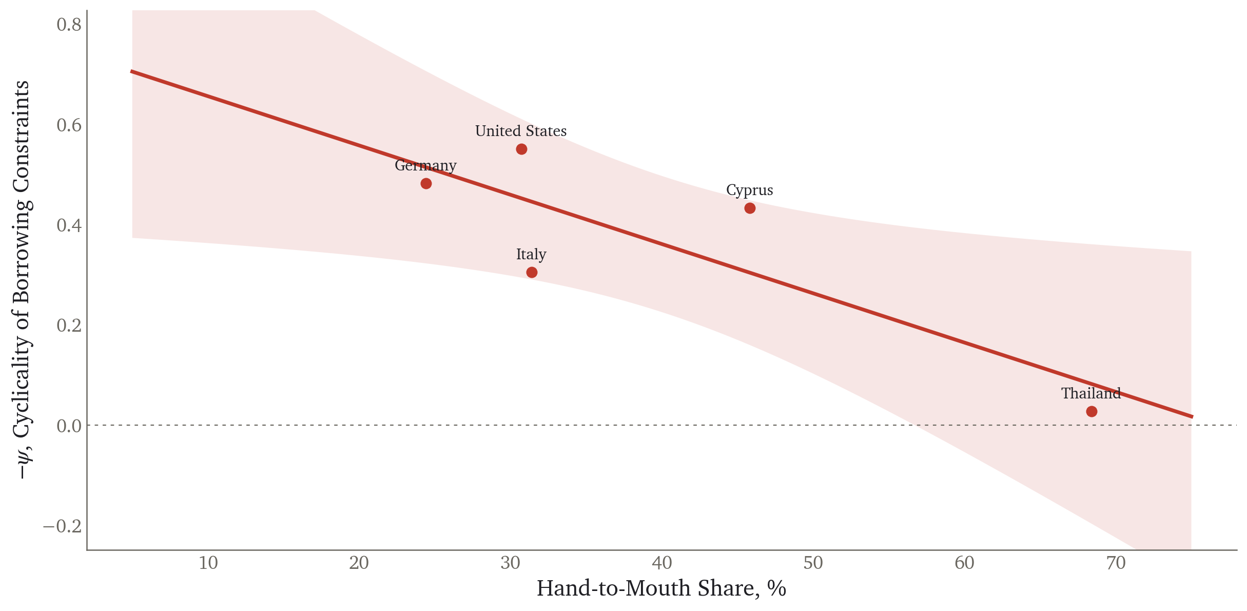
where $\mathcal{J}^{\mathbf{C},\mathbf{Y}}_{t,s},\, \mathcal{J}^{\mathbf{C},\mathbf{r}}_{t,s}$ are computed via sequence-space Jacobians (Auclert et al. 21’)
Per-country income process — calibration
Replaces the common $(\rho=0.98,\;\sigma=0.8)$ with country-specific AR(1) estimates
from code/mydos/official_sigma.do. Everything else (common $\beta=0.75$,
official $\psi$ and $\zeta$, New Keynesian Block) unchanged.
$\rho_m$
$\sigma_u$
HtM target
HtM (model)
Full IRF (p.p.)
Italy
0.9876
0.67
17%
17.0%
+6.55
Cyprus
0.9814
0.81
47%
47.0%
+18.00
Thailand
0.9665
1.40
75%
75.0%
+6.42
Notes: $\rho_m$, $\sigma_u$ from monthly AR(1) with FE residualization (age, age², year FE,
gender/education) on log labor income (HFCS Qlabinc for IT, CY; TTS
Qlabinc for TH). Common $\beta=0.75$, IES$=0.5$, $\phi_\pi=1.5$, $\kappa_w=0.1$,
$n_a=500$, $n_e=11$. Country $\psi$ from official_psi.do
($\psi_{IT}=-1.01,\;\psi_{CY}=-0.42,\;\psi_{TH}=-0.05$);
country $\zeta$ from official_zeta.do
($\zeta_{IT}=-0.04,\;\zeta_{CY}=-1.66,\;\zeta_{TH}=-0.10$).
 [Werning 15']